Build an AI-Powered Anomaly Detection System for Infrastructure Metrics
observability reliability devops
System Design Deep Dive
AI Anomaly Detection for Infrastructure Metrics
Learn a dynamic baseline for every metric, then page on-call only when something is actually wrong.
Picture a hospital ward’s bedside monitors. Every patient gets the same default alarm: heart rate over 100 beats per minute triggers a page to the nurse’s station. A marathoner recovering from surgery runs a resting heart rate of 48, so 90 already means something is badly wrong for her, but the monitor stays silent until 100. Meanwhile a patient on a standard anxiety medication sits at 95 all day as a matter of course, and the monitor screams every few hours for a condition that is not an emergency at all. The fixed threshold is wrong for almost everyone, because it was never actually about the number 100, it was about what is normal for this particular patient at this particular time of day. A good ward instead learns each patient’s personal baseline and its normal daily rhythm, sleeping heart rate lower, post-meal heart rate higher, and pages a nurse only when a reading breaks that personal pattern by more than chance would explain.
Infrastructure metrics have the exact same problem, at a much larger scale. A checkout service’s request rate is not one number, it is a curve that rises every weekday morning, dips every night, spikes on paydays, and doubles during a flash sale that was planned two weeks in advance. A fixed alert threshold, “page if CPU exceeds 80%,” either fires constantly during expected peak traffic, training every engineer on the team to ignore pages, or sits so loose that it misses a real degradation that happens to occur during a quiet period. At a scale of 2 million actively monitored time series across 50,000 hosts and containers, with metrics arriving at roughly 200,000 data points per second sustained, hand-tuning a static threshold per metric is not a staffing problem, it is a mathematical impossibility, and even if it were possible, a threshold tuned for Tuesday’s traffic is already wrong by Saturday.
The naive fix, alert whenever a metric moves more than some fixed percentage from its value an hour ago, fails for a related but sharper reason: it cannot distinguish a genuine anomaly from an expected seasonal swing, and it has no concept of correlation. When a database’s connection pool actually exhausts during a real incident, that single root cause ripples outward and trips independent alerts on API latency, queue depth, error rate, and downstream service timeouts, all within the same sixty seconds. A naive system pages on-call twenty separate times for one incident, an alert storm that buries the one signal that actually matters under nineteen symptoms of it, and by the third storm in a month, engineers start silencing the entire alerting channel rather than triaging it. The forces in tension are sensitivity against noise, and per-metric precision against the operational cost of maintaining millions of individually tuned models.
We need to solve for three things simultaneously: a baseline that adapts to each metric’s own seasonal rhythm and trend rather than a single fixed number, a correlation layer that recognizes when many simultaneous anomalies are one incident rather than many separate problems and suppresses the redundant noise, and a feedback mechanism that gets measurably better at not paging engineers for the same false positive twice.
Requirements and Constraints
Functional Requirements
- Learn a dynamic baseline for every actively monitored metric, capturing daily and weekly seasonality, trend, and normal variance, without requiring an engineer to hand-configure a threshold per metric
- Score every incoming data point for how anomalous it is relative to that metric’s current baseline, in near real time
- Correlate anomalies that fire close together in time and across topologically related services into a single incident, rather than raising one alert per metric
- Suppress duplicate and downstream alerts once an incident is open, while continuing to record every underlying anomaly for the postmortem timeline
- Onboard a brand-new metric with no history by borrowing a baseline shape from statistically similar metrics until it accumulates enough history of its own
- Capture on-call feedback, acknowledged as real, marked as false positive, or snoozed, and use it to adjust future sensitivity for that metric without a manual re-tuning cycle
- Expose an API and dashboard view showing a metric’s actual value plotted against its learned expected band, so an engineer can see why an alert did or did not fire
Non-Functional Requirements
- Scale: 2,000,000 actively scored time series across roughly 50,000 hosts and containers, ingesting at approximately 200,000 data points per second sustained, with bursts to 400,000 points per second during large deploys or scaling events
- Scoring latency: p99 under 5 seconds from the time a data point is ingested to the time an anomaly score is available for it
- Alert latency: end-to-end latency from a genuine anomaly’s onset to a page reaching on-call under 60 seconds
- Noise reduction: fewer than 5% of pages sent to a human should be later labeled false positive, and the correlated, suppressed alert volume should be at least 90% lower than naive per-metric static threshold alerting would produce at this scale
- Availability: 99.9% for the real-time scoring and correlation path; a brief scoring gap should degrade to “no new anomalies detected” rather than a crash, since a missed page is worse than a delayed one but a false page trains engineers to ignore the system
- Retention: 13 months of raw and rolled-up metric history to support seasonal model training across a full year-over-year cycle, with anomaly events and incident records retained indefinitely for audit and trend analysis
- Model freshness: per-metric baseline parameters updated continuously via streaming statistics, with a full seasonal re-decomposition at least once daily per metric cluster
Constraints and Assumptions
- We are not building the metric collection agents or exporters; we assume Prometheus-compatible scrapers, OpenTelemetry SDKs, and cloud provider metric APIs already deliver labeled time series into our ingestion layer
- We are not building a general-purpose long-term time-series database from scratch; we assume an existing TSDB such as a Prometheus-compatible remote-write target already durably stores raw metrics, and this design owns a purpose-built rollup and feature store that sits alongside it for anomaly scoring
- We are not building the paging mechanics themselves, integrations with an on-call scheduling tool are a downstream consumer; this design owns the decision of whether an anomaly is worth paging a human, not how the page is delivered
- We assume a service topology graph, which service calls which, already exists in a service catalog or CMDB and is available to the correlation engine as a read-only input
- We assume metric label cardinality is bounded by an existing ingestion-time cardinality limiter; unbounded label explosion is a separate problem this design does not attempt to solve
High-Level Architecture
The system has five major components: the Metrics Ingestion Pipeline, the Baseline Modeling Engine, the Real-Time Anomaly Scorer, the Alert Correlation and Suppression Engine, and the Feedback Loop Service.
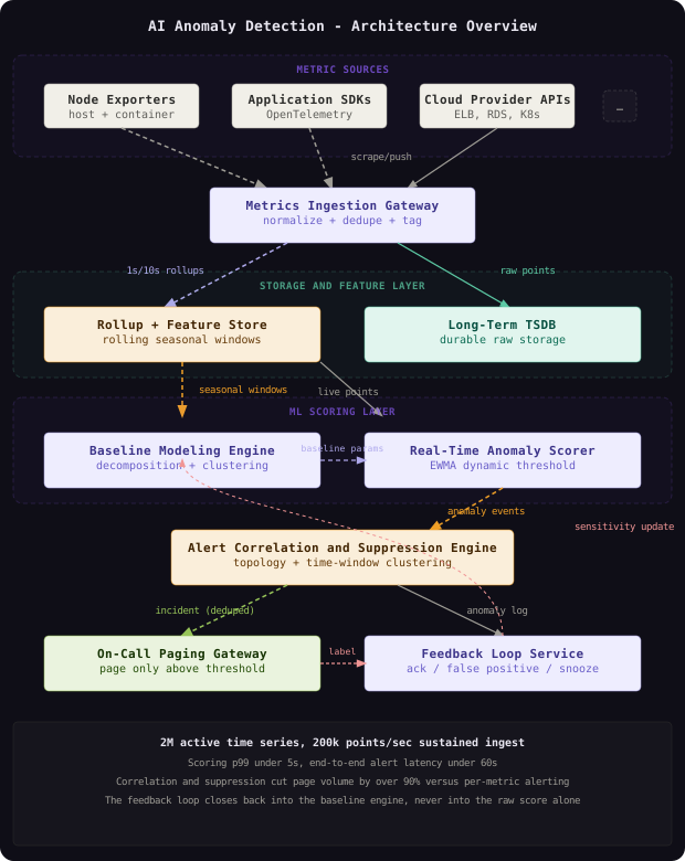
A metric data point, a host’s CPU utilization sample, a service’s request latency, arrives from an exporter or SDK and reaches the Metrics Ingestion Pipeline, which normalizes labels, deduplicates retried scrapes, and fans the point out to two destinations in the same write: a long-term time-series database for durable raw storage, and a purpose-built Rollup and Feature Store that maintains rolling seasonal windows optimized for anomaly scoring rather than dashboarding. The Baseline Modeling Engine reads from the feature store to continuously maintain, per metric, a decomposed trend, seasonal pattern, and expected variance band. The Real-Time Anomaly Scorer reads every new point alongside the current baseline for that metric and emits a score; scores that cross a metric’s dynamic threshold become anomaly events. The Alert Correlation and Suppression Engine consumes the stream of anomaly events, groups related ones into incidents using time-window and service-topology correlation, opens a suppression window so downstream symptoms of an already-known incident do not each generate a separate page, and forwards only the deduplicated incident to the paging gateway. When an engineer acknowledges, dismisses, or snoozes an alert, that action flows into the Feedback Loop Service, which adjusts the sensitivity the Baseline Modeling Engine and Anomaly Scorer apply to that metric going forward.
The full loop, from a raw metric point through scoring, correlation, paging, and feedback back into the model, is what turns this from a one-shot statistical threshold into a system that gets quieter over time without getting blind to real incidents.
The single most important architectural decision is that scoring and correlation are separate stages with separate responsibilities. The scorer’s only job is to answer “is this one data point unusual for this one metric,” a narrow, fast, statistical question. The correlation engine’s job is the harder, structural question, “are these unusual data points actually one incident.” Conflating the two into a single model produces a system that is both slower to score and worse at both jobs.
Component Deep Dives
The Metrics Ingestion Pipeline
This component’s job is to take raw metric points from thousands of heterogeneous sources, normalize them into a consistent shape, and durably fan them out to both long-term storage and the anomaly detection feature store within milliseconds.
The obvious shortcut is to let the Baseline Modeling Engine and Anomaly Scorer read directly from the long-term TSDB. That fails because a TSDB optimized for dashboard queries, arbitrary label filters, long time ranges, ad hoc aggregation, is a poor fit for the access pattern anomaly scoring actually needs: the last N seasonal cycles of one specific metric, pre-aggregated into rolling windows, fetched in single-digit milliseconds for millions of metrics continuously. The ingestion pipeline instead writes once and fans out twice, so the TSDB stays focused on durable, queryable history and the feature store stays focused on low-latency rolling statistics.
# Ingestion pipeline stage definition for the metrics gateway
pipeline: metrics-ingestion-gateway
sources:
  - type: prometheus_remote_write
    listen_port: 9201
  - type: otlp_metrics
    listen_port: 4317
  - type: cloud_provider_poll
    interval_seconds: 60
normalize:
  label_order: canonical
  dedupe_window_seconds: 5
  drop_labels: ["pod_ip", "trace_id"]
  cardinality_guard:
    max_series_per_metric_name: 500000
    action_on_breach: drop_and_alert
fanout:
  - sink: tsdb_remote_write
    target: long-term-tsdb:9090
    mode: raw
  - sink: rollup_feature_store
    target: feature-store-cluster:7000
    mode: windowed
    windows_seconds: [10, 60, 300]
partitioning:
  key: metric_id
  partitions: 256
  consumer_group: ingestion-workers
Partitioning by metric_id across 256 partitions is what lets every downstream stage, rollup computation, baseline modeling, scoring, process a given metric’s points in strict arrival order without a distributed lock, since one metric’s entire history always lands on the same partition. Deduplication within a 5 second window absorbs the retried scrapes that happen when a Prometheus exporter times out and a scrape client retries, which would otherwise register as a burst of identical values and quietly bias the seasonal model’s variance estimate.
A metric whose label set includes something high-cardinality by mistake, a raw user ID or a UUID accidentally attached as a label, can silently explode from one time series into millions within minutes. Without the cardinality_guard dropping and alerting on the breach at ingestion time, that single misconfigured exporter can overwhelm the feature store and starve baseline computation for every other metric sharing its partition.
Prometheus and its remote-write ecosystem, along with Datadog’s ingestion pipeline, both enforce cardinality limits at the point of ingestion rather than downstream, because a cardinality explosion is far cheaper to reject at the edge than to absorb and then clean up after it has already fanned out to every consumer.
The Baseline Modeling Engine
This component’s job is to maintain, for every metric, a continuously updated model of what “normal” looks like, decomposed into trend, seasonal pattern, and expected variance, so the scorer has something precise to compare against.
The tempting shortcut is a single fixed threshold per metric, set once by whoever created the alert. That is exactly the bedside-monitor mistake: a threshold correct for Tuesday afternoon traffic is wrong for Saturday at 3am, and nobody revisits it until it either pages too often and gets muted, or misses a real incident because it was tuned too loose to avoid the first problem. The baseline engine instead decomposes each metric’s recent history into three components, a slow-moving trend, a repeating seasonal pattern, and the residual noise left after removing both, and only the residual gets compared against an anomaly threshold.
Seasonal decomposition. A metric like request rate is not noise around a flat line, it is trend plus a repeating daily or weekly shape plus noise. We decompose it using a classical moving-average decomposition, robust to the kind of short gaps and spikes that real infrastructure data always has:
# Classical seasonal-trend decomposition: separates a metric's history into
# trend, seasonal pattern, and residual, using a centered moving average
# for trend and period-indexed medians for the seasonal component
import statistics
from typing import List

def moving_average_trend(values: List[float], period: int) -> List[float]:
    # Centered moving average smooths out both noise and the seasonal
    # cycle itself, leaving only the slow-moving trend
    n = len(values)
    half = period // 2
    trend = [None] * n
    for i in range(half, n - half):
        window = values[i - half: i + half + 1]
        trend[i] = sum(window) / len(window)
    return trend

def seasonal_component(values: List[float], trend: List[float], period: int) -> List[float]:
    # Detrend, then take the median deviation for each position in the
    # seasonal cycle (e.g. each hour-of-week), median is robust to the
    # occasional real incident polluting the seasonal estimate
    detrended_by_phase = {phase: [] for phase in range(period)}
    for i, (v, t) in enumerate(zip(values, trend)):
        if t is None:
            continue
        detrended_by_phase[i % period].append(v - t)
    seasonal_by_phase = {
        phase: statistics.median(diffs) if diffs else 0.0
        for phase, diffs in detrended_by_phase.items()
    }
    return [seasonal_by_phase[i % period] for i in range(len(values))]

def decompose(values: List[float], period: int) -> dict:
    trend = moving_average_trend(values, period)
    seasonal = seasonal_component(values, trend, period)
    residual = [
        v - (t if t is not None else v) - s
        for v, t, s in zip(values, trend, seasonal)
    ]
    return {"trend": trend, "seasonal": seasonal, "residual": residual}
For a metric sampled every 60 seconds with a strong daily rhythm, period is 1440 (points per day); for one with a weekly rhythm layered on top, we run the decomposition twice, once against a daily period on the detrended series and once against a weekly period, and sum both seasonal components. Using the median rather than the mean for each phase’s typical deviation is what keeps one bad day, an actual outage that happened to land on a Tuesday three weeks ago, from permanently biasing what “normal Tuesday” means going forward.
The property that makes seasonal decomposition useful for alerting, rather than just for reporting, is that the anomaly threshold gets applied to the residual, not the raw value. A raw value of 50,000 requests per second is neither normal nor abnormal on its own, it depends entirely on whether it is 2pm on a weekday or 3am on a Sunday. Only after subtracting the trend and the expected seasonal shape does “unusual” become a well-defined statistical question.
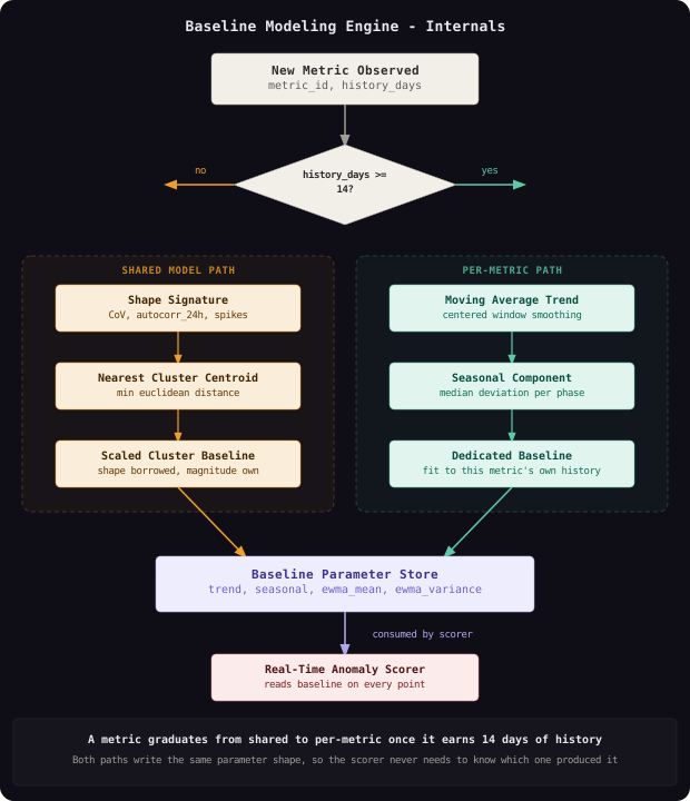
Per-metric versus shared model. Running a full seasonal decomposition independently for 2 million time series, continuously, is expensive, and a metric that started five minutes ago has no history to decompose at all. Not every metric needs, or can support, its own independently trained model. We cluster metrics by shape similarity, computed from a small feature vector (coefficient of variation, autocorrelation at 24 hours, spike frequency), and metrics that cluster together share a baseline model shape, scaled to each individual metric’s own magnitude.
# Assigns a metric to either its own dedicated baseline model or a shared
# cluster model, based on available history and shape similarity
from dataclasses import dataclass
from typing import Optional

@dataclass
class MetricProfile:
    metric_id: str
    history_days: float
    coefficient_of_variation: float
    autocorr_24h: float
    spike_frequency: float

MIN_HISTORY_DAYS_FOR_DEDICATED_MODEL = 14

def shape_signature(profile: MetricProfile) -> tuple:
    # A coarse fingerprint used to find the nearest existing cluster;
    # bucketed rather than continuous so near-identical metrics collapse
    # into the same cluster instead of each spawning a new one
    return (
        round(profile.coefficient_of_variation, 1),
        round(profile.autocorr_24h, 1),
        round(profile.spike_frequency, 2),
    )

def assign_model(
    profile: MetricProfile,
    cluster_centroids: dict,   # {cluster_id: MetricProfile}
) -> dict:
    if profile.history_days >= MIN_HISTORY_DAYS_FOR_DEDICATED_MODEL:
        return {"model_type": "per_metric", "cluster_id": None}

    best_cluster, best_distance = None, float("inf")
    for cluster_id, centroid in cluster_centroids.items():
        distance = (
            (profile.coefficient_of_variation - centroid.coefficient_of_variation) ** 2
            + (profile.autocorr_24h - centroid.autocorr_24h) ** 2
            + (profile.spike_frequency - centroid.spike_frequency) ** 2
        ) ** 0.5
        if distance < best_distance:
            best_cluster, best_distance = cluster_id, distance

    return {"model_type": "shared_cluster", "cluster_id": best_cluster}
A brand-new metric on a freshly deployed service gets assigned to whichever existing cluster its early shape most resembles, “bursty request-rate-shaped metrics” or “smooth saturation-shaped metrics,” and inherits that cluster’s seasonal shape and variance envelope immediately, scaled to its own observed magnitude. Once it accumulates 14 days of its own history, it graduates to a dedicated per-metric model that reflects its actual behavior rather than an approximation borrowed from its neighbors.
Running a dedicated model for every metric from day one sounds more accurate, but at 2 million time series it means 2 million independent decomposition jobs competing for the same compute budget, and a cold-start metric with an hour of history produces a garbage seasonal estimate no matter how much compute you throw at it. The shared-cluster fallback is not a compromise, it is what makes accurate scoring possible for a metric’s first two weeks of existence, which is exactly the period a fixed threshold would otherwise leave completely unprotected.
Datadog’s Watchdog and Amazon’s CloudWatch Anomaly Detection both use this same hybrid approach in practice, a per-metric statistical model once sufficient history exists, falling back to a coarser, shared behavioral profile for newly onboarded or low-traffic metrics, rather than either forcing every metric into one global model or requiring weeks of silence before any metric gets protected at all.
The Real-Time Anomaly Scorer
This component’s job is to take every new data point, compare it against its metric’s current baseline, and emit a score in near real time, without becoming the bottleneck that everything else is waiting on.
Dynamic threshold modeling. A static band, “alert if the value is more than 3 units away from the mean,” breaks the moment a metric’s variance itself changes with the time of day, which it almost always does, request latency is tighter at 3am with little traffic and naturally noisier at peak load with more concurrent connections. The threshold has to widen and narrow with the metric’s own expected variance, not stay fixed.
# Dynamic threshold scoring: maintains an exponentially weighted mean and
# variance of the seasonally-adjusted residual, and scores new points
# against a band that widens or narrows with the metric's own volatility
from dataclasses import dataclass

@dataclass
class EwmaState:
    mean: float
    variance: float
    initialized: bool = False

EWMA_ALPHA = 0.06          # weight given to each new observation
MIN_VARIANCE_FLOOR = 1e-6  # guards against a division by near-zero on flat metrics

def update_ewma(state: EwmaState, residual: float) -> EwmaState:
    if not state.initialized:
        return EwmaState(mean=residual, variance=0.0, initialized=True)
    delta = residual - state.mean
    new_mean = state.mean + EWMA_ALPHA * delta
    new_variance = (1 - EWMA_ALPHA) * (state.variance + EWMA_ALPHA * delta * delta)
    return EwmaState(mean=new_mean, variance=new_variance, initialized=True)

def score_point(
    raw_value: float,
    trend_estimate: float,
    seasonal_estimate: float,
    residual_state: EwmaState,
    sensitivity_multiplier: float = 1.0,
) -> dict:
    residual = raw_value - trend_estimate - seasonal_estimate
    std_dev = max(residual_state.variance, MIN_VARIANCE_FLOOR) ** 0.5
    z_score = residual / std_dev if std_dev > 0 else 0.0

    # sensitivity_multiplier is adjusted per metric by the feedback loop,
    # widening the effective band for metrics with a history of false positives
    effective_threshold = 3.5 * sensitivity_multiplier
    is_anomaly = abs(z_score) > effective_threshold

    return {
        "residual": residual,
        "z_score": z_score,
        "expected_band_low": trend_estimate + seasonal_estimate - effective_threshold * std_dev,
        "expected_band_high": trend_estimate + seasonal_estimate + effective_threshold * std_dev,
        "is_anomaly": is_anomaly,
        "severity": "critical" if abs(z_score) > effective_threshold * 1.7 else "warning",
    }
EWMA_ALPHA controls how quickly the band adapts, a small value like 0.06 means the band reacts to a genuine, sustained level shift over roughly fifteen to twenty data points rather than either ignoring it for hours or over-fitting to a single spike. sensitivity_multiplier starts at 1.0 for every metric and is the exact lever the feedback loop turns, widening it for a metric that keeps generating false positives without touching the underlying statistical model at all.
The property that makes exponentially weighted variance the right choice here, over a fixed-window standard deviation, is that it never needs to store or replay a window of raw history to update, one multiply-add per point, which is what makes scoring 200,000 points per second on commodity compute feasible in the first place.
A residual variance that has genuinely collapsed to near zero, a metric that has been perfectly flat for days, makes even a tiny absolute change register as an enormous z-score. The MIN_VARIANCE_FLOOR exists specifically to prevent a one-unit blip on an otherwise dead-flat metric from producing a false “10-sigma” anomaly that looks alarming on a dashboard but reflects nothing more than division by a number very close to zero.
Facebook’s production monitoring stack and Netflix’s Atlas both describe exponentially weighted moving statistics as their default choice for streaming anomaly bands over fixed sliding windows, precisely because the constant-memory, single-pass update is what makes per-metric statistical scoring tractable at millions of concurrent time series.
The Alert Correlation and Suppression Engine
This component’s job is to take a stream of individually scored anomalies and decide which ones are actually the same underlying incident, so on-call gets paged once per incident, not once per symptom.
The naive approach forwards every anomaly straight to paging. During a real database connection pool exhaustion, that single root cause typically trips ten to twenty independent metric anomalies within the same minute, API latency, error rate, queue depth, thread pool saturation, and every downstream service’s own latency, each fires its own alert. Twenty pages for one incident is not twenty times more information, it is one piece of information buried under nineteen duplicates, and it is precisely the pattern that trains an on-call rotation to silence the whole channel.
Multi-metric correlation. We group anomalies into incidents using two independent signals combined: how close together in time they fired, and how close together they sit in the service dependency graph.
# Groups near-simultaneous anomalies into incidents using union-find,
# merging anomalies that are close in time AND connected in the service
# topology graph, or strongly cross-correlated in their residual series
from collections import defaultdict

class UnionFind:
    def __init__(self, ids):
        self.parent = {i: i for i in ids}

    def find(self, x):
        while self.parent[x] != x:
            self.parent[x] = self.parent[self.parent[x]]
            x = self.parent[x]
        return x

    def union(self, a, b):
        ra, rb = self.find(a), self.find(b)
        if ra != rb:
            self.parent[ra] = rb

TIME_WINDOW_SECONDS = 90

def topology_connected(service_a: str, service_b: str, topology_edges: set) -> bool:
    return (service_a, service_b) in topology_edges or (service_b, service_a) in topology_edges

def correlate_anomalies(anomalies: list, topology_edges: set) -> list:
    # anomalies: [{"event_id", "metric_id", "service", "ts", "residual_series"}, ...]
    uf = UnionFind([a["event_id"] for a in anomalies])
    anomalies_sorted = sorted(anomalies, key=lambda a: a["ts"])

    for i, a in enumerate(anomalies_sorted):
        for b in anomalies_sorted[i + 1:]:
            if b["ts"] - a["ts"] > TIME_WINDOW_SECONDS:
                break
            same_service = a["service"] == b["service"]
            connected = topology_connected(a["service"], b["service"], topology_edges)
            if same_service or connected:
                uf.union(a["event_id"], b["event_id"])

    groups = defaultdict(list)
    for a in anomalies_sorted:
        groups[uf.find(a["event_id"])].append(a)
    return list(groups.values())
Sorting by timestamp first turns what would otherwise be an all-pairs comparison across every anomaly into a bounded sliding window, since the inner loop breaks as soon as it walks past the 90 second correlation window, making the common case close to linear in the number of anomalies rather than quadratic. Two anomalies merge into the same incident either because they hit the same service, or because the topology graph shows a direct dependency edge between their services, a payments service’s error spike and its database’s connection pool spike merge because the topology graph knows one calls the other.
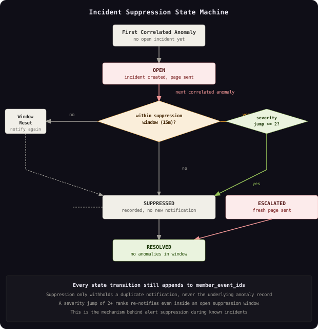
Alert suppression during incidents. Once a group of anomalies opens an incident, every additional anomaly that correlates into that same group within the suppression window gets recorded but does not generate a new page, and the incident escalates only if its severity genuinely worsens.
# Incident suppression state machine: opens an incident on first correlated
# anomaly, suppresses duplicate pages for related anomalies, and only
# re-notifies if the incident's severity meaningfully escalates
from datetime import datetime, timedelta
from enum import Enum

class IncidentStatus(Enum):
    OPEN = "open"
    SUPPRESSED = "suppressed"
    ESCALATED = "escalated"
    RESOLVED = "resolved"

SUPPRESSION_WINDOW = timedelta(minutes=15)
ESCALATION_SEVERITY_JUMP = 2   # e.g. warning (1) -> critical (3)

SEVERITY_RANK = {"warning": 1, "critical": 3}

class Incident:
    def __init__(self, incident_id: str, opened_at: datetime, initial_severity: str):
        self.incident_id = incident_id
        self.opened_at = opened_at
        self.status = IncidentStatus.OPEN
        self.max_severity_rank = SEVERITY_RANK[initial_severity]
        self.member_event_ids = []
        self.last_notified_at = opened_at

    def absorb_anomaly(self, event_id: str, severity: str, now: datetime) -> bool:
        # Returns True if this anomaly should trigger a fresh notification
        self.member_event_ids.append(event_id)
        incoming_rank = SEVERITY_RANK[severity]
        within_window = (now - self.last_notified_at) < SUPPRESSION_WINDOW

        if not within_window:
            self.last_notified_at = now
            self.max_severity_rank = max(self.max_severity_rank, incoming_rank)
            return True

        if incoming_rank - self.max_severity_rank >= ESCALATION_SEVERITY_JUMP:
            self.status = IncidentStatus.ESCALATED
            self.max_severity_rank = incoming_rank
            self.last_notified_at = now
            return True

        self.status = IncidentStatus.SUPPRESSED
        self.max_severity_rank = max(self.max_severity_rank, incoming_rank)
        return False
The suppression window resets on genuine escalation, not on a timer alone, so a page that has already gone out for a warning-level database slowdown does not fully suppress a second, distinct page fifteen minutes later when that same incident escalates into a critical outage. Every absorbed anomaly is still recorded against member_event_ids, so the postmortem timeline shows the full blast radius even though on-call only received one or two actual notifications.
The property that makes suppression safe rather than dangerous is that it suppresses notifications, never data. Every correlated anomaly is still scored, timestamped, and stored against the incident record. Suppression only changes whether a human gets paged again for information that would not have changed their response, it never hides the anomaly from the system itself.
Correlating purely on time-window overlap, without the topology graph, produces false merges during broad, unrelated events, a scheduled deploy across dozens of unrelated services can trigger simultaneous, purely coincidental anomalies that get incorrectly bundled into one incident, masking the fact that they are actually independent problems needing independent responses.
PagerDuty’s event intelligence and Google’s production monitoring both describe topology-aware grouping, correlating alerts by service dependency graph in addition to time proximity, as the specific change that took their alert-to-incident ratio from double digits down to close to one-to-one during real outages.
The Feedback Loop Service
This component’s job is to turn an on-call engineer’s acknowledgment, dismissal, or snooze of an alert into a measurable, automatic adjustment to that metric’s future sensitivity, so the same false positive does not have to be manually re-tuned every time it recurs.
The shortcut most teams reach for is a shared support queue where engineers complain about noisy alerts and someone eventually gets around to manually raising a threshold. That does not scale past a handful of hand-picked, high-visibility alerts, and it means every metric’s sensitivity is only as good as the last time someone remembered to look at it. Feedback loop on false positives has to be structural: every label an engineer attaches to an alert becomes training signal the very next time that metric is scored.
# Bayesian-flavored sensitivity adjustment: nudges a metric's threshold
# multiplier based on the running ratio of true-positive to false-positive
# feedback, bounded so a burst of feedback cannot overcorrect in one step
from dataclasses import dataclass

@dataclass
class FeedbackState:
    true_positive_count: float
    false_positive_count: float
    sensitivity_multiplier: float

FEEDBACK_DECAY = 0.98         # older feedback counts for slightly less over time
MIN_MULTIPLIER = 0.6          # never let a metric become more than ~1.7x more sensitive
MAX_MULTIPLIER = 3.0          # never let a metric become numb beyond a 3x wider band
ADJUSTMENT_STEP = 0.08

def apply_feedback(state: FeedbackState, label: str) -> FeedbackState:
    # label is "true_positive", "false_positive", or "snoozed"
    tp = state.true_positive_count * FEEDBACK_DECAY
    fp = state.false_positive_count * FEEDBACK_DECAY
    multiplier = state.sensitivity_multiplier

    if label == "false_positive":
        fp += 1
        multiplier = min(MAX_MULTIPLIER, multiplier + ADJUSTMENT_STEP)
    elif label == "true_positive":
        tp += 1
        # A true positive is evidence the current sensitivity is working;
        # nudge gently back toward 1.0 rather than snapping instantly,
        # so a single confirmed page doesn't erase weeks of learned tolerance
        multiplier = max(MIN_MULTIPLIER, multiplier - ADJUSTMENT_STEP * 0.4)
    elif label == "snoozed":
        # Weaker signal than an explicit false positive, still nudges
        # sensitivity slightly since a snooze means "not urgent right now"
        fp += 0.4
        multiplier = min(MAX_MULTIPLIER, multiplier + ADJUSTMENT_STEP * 0.3)

    return FeedbackState(
        true_positive_count=tp,
        false_positive_count=fp,
        sensitivity_multiplier=round(multiplier, 3),
    )

def false_positive_rate(state: FeedbackState) -> float:
    total = state.true_positive_count + state.false_positive_count
    return state.false_positive_count / total if total > 0 else 0.0
sensitivity_multiplier flows directly into the score_point function shown earlier, so a metric that has accumulated a run of false positives widens its own effective band without an engineer opening a config file, while MIN_MULTIPLIER and MAX_MULTIPLIER cap how far a single burst of feedback, or a single overzealous engineer mass-dismissing alerts during an unrelated noisy afternoon, can swing sensitivity in one direction. FEEDBACK_DECAY ensures feedback from six months ago carries less weight than feedback from this week, since the metric’s own behavior, and the model’s baseline accuracy, both drift over time.
The property that makes this feedback loop safe is that it is bounded and asymmetric, not a free-running control loop. A run of false positives can only ever widen the band up to MAX_MULTIPLIER, never disable alerting for a metric entirely, and a single true positive pulls sensitivity back gently rather than snapping it to full strength, which prevents the exact oscillation, too sensitive, then too numb, then too sensitive again, that an unbounded feedback controller would produce.
If false-positive feedback is accepted with no accountability for who submitted it, a team under pressure during an unrelated noisy week can mass-dismiss real alerts to make the paging stop, quietly numbing a metric right before the incident that alert was designed to catch. Attribute every feedback label to an engineer and a timestamp, and flag any metric whose sensitivity multiplier moves sharply in a short window for a human review before the next model refresh.
New Relic’s and Datadog’s anomaly detection products both expose an explicit “was this alert useful” feedback action for exactly this reason, and both describe per-alert sensitivity tuning as the single biggest lever for reducing the alert fatigue that causes teams to abandon anomaly detection features within the first few months of adoption.
Data Model
The durable state splits into the metric catalog and cluster assignments the Baseline Modeling Engine depends on, the anomaly and incident records the Correlation Engine produces, and the feedback labels that close the loop.
-- Metric catalog: every actively tracked time series and its current model assignment
CREATE TABLE metric_catalog (
    metric_id          BIGSERIAL PRIMARY KEY,
    metric_name          TEXT NOT NULL,
    labels                 JSONB NOT NULL,
    service_id               TEXT NOT NULL,
    unit                       TEXT NOT NULL,
    resolution_seconds           SMALLINT NOT NULL DEFAULT 60,
    first_seen_at                  TIMESTAMPTZ NOT NULL DEFAULT NOW(),
    history_days                     NUMERIC(8,2) NOT NULL DEFAULT 0,
    model_type                         TEXT NOT NULL DEFAULT 'shared_cluster'
                                        CHECK (model_type IN ('per_metric', 'shared_cluster')),
    cluster_id                           BIGINT,
    sensitivity_multiplier                 NUMERIC(4,3) NOT NULL DEFAULT 1.000,
    UNIQUE (metric_name, labels)
);
CREATE INDEX ON metric_catalog (service_id);
CREATE INDEX ON metric_catalog (cluster_id) WHERE model_type = 'shared_cluster';

-- Shared cluster centroids used for cold-start baseline assignment
CREATE TABLE metric_clusters (
    cluster_id            BIGSERIAL PRIMARY KEY,
    shape_signature          JSONB NOT NULL,
    member_count                INTEGER NOT NULL DEFAULT 0,
    trained_at                    TIMESTAMPTZ NOT NULL DEFAULT NOW()
);

-- Baseline model parameters, versioned so a bad retrain can be rolled back
CREATE TABLE baseline_models (
    model_version_id      BIGSERIAL PRIMARY KEY,
    metric_id               BIGINT REFERENCES metric_catalog(metric_id),
    cluster_id                 BIGINT REFERENCES metric_clusters(cluster_id),
    trend_params                 JSONB NOT NULL,
    seasonal_params                JSONB NOT NULL,
    ewma_mean                        DOUBLE PRECISION NOT NULL DEFAULT 0,
    ewma_variance                      DOUBLE PRECISION NOT NULL DEFAULT 0,
    valid_from                           TIMESTAMPTZ NOT NULL DEFAULT NOW(),
    CHECK (metric_id IS NOT NULL OR cluster_id IS NOT NULL)
);
CREATE INDEX ON baseline_models (metric_id, valid_from DESC);

-- Individual anomaly events, the raw signal before correlation
CREATE TABLE anomaly_events (
    event_id             BIGSERIAL PRIMARY KEY,
    metric_id              BIGINT NOT NULL REFERENCES metric_catalog(metric_id),
    ts                        TIMESTAMPTZ NOT NULL,
    observed_value               DOUBLE PRECISION NOT NULL,
    expected_low                    DOUBLE PRECISION NOT NULL,
    expected_high                     DOUBLE PRECISION NOT NULL,
    z_score                             DOUBLE PRECISION NOT NULL,
    severity                              TEXT NOT NULL CHECK (severity IN ('warning', 'critical')),
    incident_id                             BIGINT
) PARTITION BY RANGE (ts);
CREATE INDEX ON anomaly_events (metric_id, ts DESC);
CREATE INDEX ON anomaly_events (incident_id) WHERE incident_id IS NOT NULL;

-- Correlated incidents, the deduplicated unit that actually pages a human
CREATE TABLE incidents (
    incident_id           BIGSERIAL PRIMARY KEY,
    opened_at                TIMESTAMPTZ NOT NULL,
    closed_at                   TIMESTAMPTZ,
    status                         TEXT NOT NULL DEFAULT 'open'
                                    CHECK (status IN ('open', 'suppressed', 'escalated', 'resolved')),
    root_service_id                    TEXT,
    max_severity                          TEXT NOT NULL,
    member_event_count                       INTEGER NOT NULL DEFAULT 0,
    notification_count                          INTEGER NOT NULL DEFAULT 0
);

-- Engineer-submitted labels that drive the feedback loop
CREATE TABLE feedback_labels (
    feedback_id           BIGSERIAL PRIMARY KEY,
    incident_id              BIGINT REFERENCES incidents(incident_id),
    metric_id                   BIGINT REFERENCES metric_catalog(metric_id),
    label                          TEXT NOT NULL CHECK (label IN ('true_positive', 'false_positive', 'snoozed')),
    engineer_id                       TEXT NOT NULL,
    submitted_at                        TIMESTAMPTZ NOT NULL DEFAULT NOW()
);
CREATE INDEX ON feedback_labels (metric_id, submitted_at DESC);
anomaly_events is range-partitioned by ts, so a query for “anomalies in the last 24 hours” prunes every older partition before scanning a row, which matters at the ingestion volume this system sustains. The sharding key across the whole system is metric_id, the ingestion partitions, the feature store’s rolling windows, and baseline_models all key on it, so one metric’s entire lifecycle, from its first data point through every baseline retrain, lives behind a single logical key even though the physical storage spans a stream partition, a feature store shard, and a relational table.
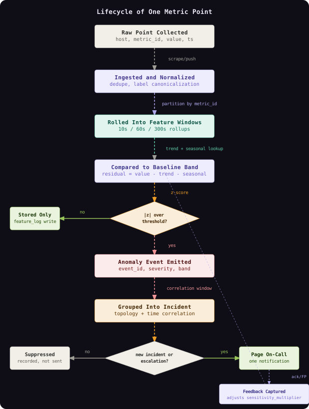
Storing expected_low and expected_high directly on every anomaly_events row, not just the score, is what makes the dashboard view showing “here’s what we expected versus what happened” possible without re-running the baseline model after the fact. An anomaly record that only stores a z-score forces every downstream consumer to re-derive the band from historical baseline state, which is slower and, worse, gives a different answer if the baseline has since been retrained.
Key Algorithms and Protocols
The core algorithms, seasonal decomposition, EWMA-based dynamic thresholding, union-find correlation, and bounded feedback adjustment, are covered in depth in their respective component sections above, since each one only makes sense alongside the component whose job it solves. Two properties tie them together as a system rather than four independent tools.
First, every algorithm operates on the residual after removing trend and seasonality, never on the raw value. This is what lets a single z_score > threshold comparison work correctly whether the metric is CPU utilization, error rate, or queue depth, because by the time any algorithm sees the number, it has already been normalized into “how many standard deviations from what we expected right now,” a unit that means the same thing across every metric shape in the system.
Second, every algorithm is designed to run as an incremental, constant-memory update per data point rather than a batch recomputation over history. The EWMA update, the union-find merge within a bounded time window, and the feedback multiplier adjustment all touch a small, fixed amount of state per event. At 200,000 points per second sustained across 2 million time series, any algorithm that requires re-scanning history on every new point is not a slower version of the same design, it is a different, infeasible design.
The property that makes this whole pipeline scale linearly with ingestion volume, rather than with the size of retained history, is that every stage after ingestion operates on a fixed-size summary of the past, an EWMA state, a cluster centroid, a sensitivity multiplier, never on the raw history itself. History lives in the feature store for humans to inspect; the hot path never reads it.
Scaling and Performance
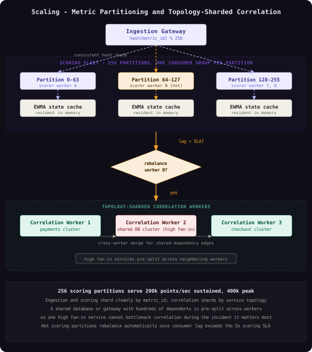
The system scales along the same partitioning key end to end. The ingestion pipeline’s 256 metric_id partitions determine parallelism for the Baseline Modeling Engine and Anomaly Scorer, both of which run as a consumer group reading those same partitions, so adding scoring capacity is a matter of adding consumers up to the partition count, not a re-architecture. The Correlation Engine is the one component that cannot shard purely by metric_id, because correlating anomalies requires seeing every anomaly from topologically related services within the same time window, so it shards instead by service-topology cluster, pre-computed offline so that services likely to correlate land on the same correlation worker.
Capacity Estimation:

Given:
  - 2,000,000 actively scored time series across ~50,000 hosts/containers
  - Ingestion: 200,000 points/sec sustained, 400,000 points/sec peak
  - Average point size after label normalization: ~60 bytes raw
  - Anomaly rate: roughly 0.1% of scored points cross the dynamic threshold
  - Correlation window: 90 seconds, average incident absorbs ~12 correlated anomalies

Ingestion and scoring path:
  Sustained throughput: 200,000 points/sec * 60 bytes = 12MB/sec raw ingest
  Peak throughput: 400,000 points/sec * 60 bytes = 24MB/sec raw ingest
  EWMA state per metric: ~48 bytes (mean, variance, timestamps, multiplier)
  Total scorer working set: 2,000,000 * 48 bytes ~= 96MB, comfortably memory-resident per shard

Anomaly and incident volume:
  Raw anomaly events/day: 200,000/sec * 86,400 * 0.001 ~= 17,280,000/day
  Incidents/day after correlation (avg 12 anomalies/incident): 17,280,000 / 12 ~= 1,440,000/day
  Notifications/day after suppression (avg 1.4 notifications/incident): ~2,016,000/day
  Note: notification count above is pre-severity-filtering; only critical-severity
  incidents page a human, roughly 3% of correlated incidents, ~43,000 pages/day
  system-wide, dominated by large multi-tenant platforms; a single team's on-call
  rotation typically owns a few dozen of these per day at most

Storage:
  anomaly_events row size (~90 bytes): 17,280,000 * 90 bytes ~= 1.5GB/day
  13-month retention: 1.5GB * 395 days ~= 605GB for anomaly event history
  Rollup feature store (10s/60s/300s windows, 2M metrics): ~40GB resident working set
Correlation workers are the most likely bottleneck under this design, since the topology-sharded assignment means a single, highly-connected service, a shared database or an API gateway with hundreds of dependents, can concentrate a disproportionate share of correlation work on one worker during a real incident, precisely the moment correlation matters most. The mitigation mirrors how a hot shard is handled anywhere else: pre-split the highest-fan-in services’ topology neighborhoods across multiple correlation workers ahead of time, with a lightweight cross-worker merge step for the rare anomaly pair that lands on different workers, rather than waiting for an incident to reveal the imbalance.
Google’s Monarch monitoring system and Meta’s internal alerting pipeline both report that correlation and grouping, not raw metric ingestion, is the component that requires the most careful sharding attention at scale, because ingestion partitions cleanly by an independent key while correlation inherently needs visibility across a graph that does not partition as cleanly.
Failure Modes and Recovery
| Failure | Detection | Impact | Recovery |
|---|---|---|---|
| Ingestion partition consumer lag spike | Consumer lag alarm per partition, compared against the 5 second scoring SLA | Anomaly scoring for metrics on that partition falls behind, delaying detection | Autoscale scoring consumers up to the partition count, apply backpressure to the slowest sources, page if lag exceeds the SLA for more than 2 minutes |
| Baseline model retrain produces a corrupted seasonal estimate | Sanity check comparing new model’s expected band width against the prior version before activation | A metric could either alert constantly or go silent if the bad model is promoted | Reject the retrain if band width changes by more than a configured bound versus the previous version; keep serving the last known-good baseline_models row |
| Correlation engine worker failure | Health check and heartbeat on each topology-sharded worker | Anomalies for that worker’s service cluster stop correlating, risking an alert storm instead of one incident | Failover to a standby worker holding the same topology shard assignment; anomalies queue briefly rather than being dropped |
| Feedback loop poisoning from mass alert dismissal | Anomaly detector flags a sharp, short-window swing in a metric’s sensitivity_multiplier | That metric could go numb right before a real incident it was tuned to catch | Cap per-window multiplier movement, require a second engineer’s confirmation for any metric whose sensitivity moves past a configured threshold in under an hour |
| Metric cardinality explosion on one source | Cardinality guard at ingestion, alert on series-per-metric-name breach | Feature store and scoring capacity for that partition gets starved, delaying unrelated metrics sharing it | Drop and quarantine the offending label combination at ingestion, alert the owning team, backfill once the source is fixed |
| Clock skew between hosts reporting metrics | Timestamp bounds check comparing reported time against server-observed ingest time | Seasonal phase assignment and correlation time windows compute against the wrong moment | Reject and quarantine points with timestamps outside an acceptable skew window, alert the host, do not silently accept them as on-time |
The most common operational mistake is treating a quiet alerting channel as evidence the system is working well, rather than checking whether it went quiet because incidents stopped or because sensitivity silently drifted numb. Track the false-negative signal directly, incidents discovered by an engineer before the system paged for them, as a first-class metric, not just the false-positive rate, since a system tuned only against false positives will happily converge toward saying nothing at all.
Comparison of Approaches
| Approach | Latency | Complexity | Failure Mode | Best Fit |
|---|---|---|---|---|
| Fixed static thresholds | Instant, no computation needed | Low to set up, high ongoing maintenance burden | Wrong the moment traffic patterns shift; requires constant manual re-tuning per metric | Small, stable metric sets where an engineer can realistically hand-tune and revisit every threshold |
| Per-metric statistical model (seasonal decomposition + EWMA) | Sub-second scoring, daily retrain cycle | Medium, one model per metric but each is cheap and interpretable | Needs 1-2 weeks of history to become accurate; degrades on metrics with irregular, non-seasonal behavior | The default choice for infrastructure metrics with clear daily or weekly rhythm at large scale |
| Shared cluster model | Sub-second scoring, shared retrain across a cluster | Low, far fewer models to maintain than per-metric | Less precise for a metric whose true behavior diverges from its cluster’s centroid shape | Cold-start coverage for new or low-traffic metrics until they earn a dedicated model |
| Deep learning sequence model (e.g. LSTM autoencoder per metric family) | Higher inference latency, expensive retraining | High, requires GPU infrastructure, labeled data, and careful drift monitoring | Opaque failures that are hard to explain to an on-call engineer at 3am; overfits without abundant clean training data | Complex, non-seasonal, multivariate metrics where simple decomposition genuinely fails to capture the pattern |
| Rule-based percent-change alerting | Instant | Very low | Cannot distinguish an expected seasonal jump from a genuine anomaly; extremely noisy | Rapid prototyping only, or as a temporary stopgap before a real baseline model is in place |
For infrastructure metrics at the scale described here, the per-metric statistical model with a shared-cluster fallback for cold start is the right default. It clears the 5 second scoring latency requirement comfortably, stays interpretable enough that an on-call engineer can look at a dashboard and immediately see why an alert fired, and its accuracy scales with the amount of history available rather than requiring a large labeled training set upfront. A deep learning approach is worth revisiting only for a specific subset of metrics with genuinely complex, non-seasonal, multivariate behavior that decomposition demonstrably fails to capture, not as a wholesale replacement for the statistical baseline that handles the other 99% of metrics correctly and cheaply.
Key Takeaways
- Seasonal decomposition turns “unusual” into a well-defined question: comparing a raw value against a threshold is meaningless without first removing the trend and the expected seasonal shape, since a value’s normalcy depends entirely on when it occurred.
- Dynamic threshold modeling has to widen and narrow with a metric’s own volatility: a fixed band is wrong the moment traffic-driven variance itself changes across the day, which it always does.
- Model per-metric versus shared model is a spectrum, not a binary choice: dedicated models earn accuracy from history, shared cluster models provide immediate coverage for metrics that have not accumulated any yet.
- Multi-metric correlation needs topology, not just timing: two anomalies close together in time are only the same incident if the services behind them are actually connected, otherwise coincident but unrelated events get wrongly merged.
- Alert suppression during incidents must suppress notifications, never data: every correlated anomaly stays recorded for the postmortem even when it does not generate a second page.
- The feedback loop on false positives has to be bounded and attributed: unbounded sensitivity adjustment from unaccountable feedback can silently numb a metric right before the incident it exists to catch.
- Every hot-path algorithm operates on constant-size state per metric: an EWMA update, a cluster centroid, a sensitivity multiplier, never a full history replay, which is what keeps the system’s cost proportional to ingestion volume rather than retained history.
- Scoring and correlation are deliberately separate concerns: one answers a narrow statistical question about a single metric, the other answers a structural question about how many metrics tell the same story.
The counter-intuitive lesson is that making an alerting system quieter and making it more trustworthy are the same problem, not two competing goals in tension. A system that pages less often because it correlates and suppresses correctly earns back the attention it needs from on-call precisely because every page that does arrive means something, while a system that pages constantly, even if every individual alert is technically accurate, trains the humans downstream of it to stop looking, which is a worse failure mode than any single missed anomaly.
Frequently Asked Questions
Q: Why not just use fixed thresholds and have engineers tune them per metric?
A: At 2 million time series, hand-tuning is not a staffing problem you can solve by hiring more engineers, it is mathematically infeasible, and even a perfectly tuned threshold goes stale the moment traffic patterns shift, which happens continuously. A dynamic baseline that adapts to trend and seasonality automatically is the only approach whose maintenance cost does not scale linearly with the number of metrics being watched.
Q: Why not train a single global deep learning model across all metrics instead of per-metric or per-cluster statistical models?
A: A single global model has to learn the shape of every metric type simultaneously, CPU utilization, queue depth, error rate, latency, which behave completely differently, and it becomes a black box that cannot explain to an on-call engineer why a specific alert fired at 3am. The statistical decomposition approach is both cheaper to run at this scale and directly interpretable, since the expected band it computes can be plotted right next to the actual value.
Q: How does the system protect a metric with no history at all?
A: New metrics are assigned to the nearest existing shared cluster based on a coarse shape signature, coefficient of variation, autocorrelation, spike frequency, computed from even a small amount of early data, and inherit that cluster’s seasonal shape scaled to their own magnitude. Once a metric accumulates roughly two weeks of its own history it graduates to a dedicated per-metric model, so coverage exists from the first hour rather than only after a multi-week blind spot.
Q: Why not just forward every anomaly to PagerDuty and let its deduplication logic handle the noise?
A: Generic downstream deduplication tools group by alert name or a manually configured key, they have no visibility into the service topology graph or the time-correlated residual statistics that let this system recognize twenty different metric names as one root cause. Doing correlation upstream, with topology and time-window awareness purpose-built for this domain, catches merges that a generic dedup key would never express.
Q: How do you keep the feedback loop from being gamed or from silently going wrong?
A: Every feedback label is attributed to a specific engineer and timestamp, sensitivity adjustments are bounded per step and per time window, and any metric whose sensitivity multiplier moves sharply in a short period gets flagged for human review before the next model refresh rather than applied silently. The system also tracks false negatives, incidents a human found before the system alerted, as a first-class signal, so a metric quietly tuned into silence is visible in that metric rather than hidden behind a falling false-positive rate.
Q: Why decompose seasonality explicitly instead of just using a longer moving average window to smooth out daily variation?
A: A longer moving average blurs together the trend and the seasonal pattern instead of separating them, so it lags behind genuine trend shifts by however long the window is, and it cannot express “this specific hour of the week is normally quieter” the way an explicit seasonal component can. Explicit decomposition keeps the residual, and therefore the anomaly score, sensitive to real change while staying blind to the expected daily and weekly rhythm.
Interview Questions
Q: Design the baseline modeling component for a system that must track dynamic thresholds for millions of time series with varying seasonal patterns. How would you avoid retraining a full model on every new data point?
Expected depth: Discuss seasonal-trend decomposition into trend, seasonal, and residual components, using exponentially weighted moving statistics for constant-memory incremental updates instead of a sliding window replay, and the tradeoff between per-metric model accuracy and the compute cost of maintaining millions of independent models.
Q: How would you correlate anomalies across multiple related metrics into a single incident, and what happens if your correlation is wrong?
Expected depth: Discuss combining time-window proximity with a service topology graph rather than time alone, using a union-find or graph-clustering approach bounded by a correlation time window, and the operational cost of both false merges, hiding a genuinely separate incident, and false splits, generating an alert storm for one root cause.
Q: A metric was just deployed an hour ago and has no history. How does your system decide whether a data point from it is anomalous?
Expected depth: Discuss cold-start handling via a shared cluster model assigned by shape signature, the tradeoff of coarser accuracy against having any coverage at all, and the graduation criteria and process for moving a metric from a shared model to a dedicated per-metric model once sufficient history accumulates.
Q: How would you design the feedback mechanism so that on-call engineers dismissing alerts as false positives actually improves the system, without letting a bad week of feedback permanently break alerting for a metric?
Expected depth: Discuss attributing feedback to engineers and timestamps, bounding sensitivity adjustment per step and per time window, decaying older feedback so recent signal dominates without erasing history entirely, and monitoring false negatives as a counterbalance to prevent the system from optimizing purely toward silence.
Q: Walk through how you would prevent an alert storm during a real incident where one root cause trips dozens of downstream metric anomalies within the same minute.
Expected depth: Discuss opening an incident on the first correlated anomaly, suppressing further notifications for anomalies that correlate into the same incident within a suppression window, re-notifying only on genuine severity escalation rather than a fixed timer, and continuing to record every underlying anomaly even while suppressing the corresponding notification, so the postmortem timeline stays complete.
Premium Content
Unlock the full article along with everything else in the archive — all in one place.