Build Amazon's Warehouse Picking Route Optimizer


scalability distributed-systems performance

System Design Deep Dive

Warehouse Picking Route Optimizer

Batch orders, solve a walking-distance TSP across a million square feet, and re-route a picker mid-aisle without ever handing them a worse path.

⏱ 14 min read📐 Advanced🏭 Scalability

Picture a grocery shopper handed a list of forty items with no thought given to where anything sits on the shelves. They will find all forty eventually, but they will crisscross the same three aisles five or six times doing it, because the list was written in the order the items were requested, not the order they physically appear in the store. Now stretch that supermarket into a fulfillment center the size of eighteen football fields, hand the list to four hundred different shoppers at once, and scatter each list’s items across zones that can be a quarter mile apart. The cost of a badly ordered list stops being a minor inconvenience and starts being the difference between a warehouse that ships every promised order on time and one that quietly falls behind every single shift.

The hard part is not finding a path between two shelves. Any engineer can call a pathfinding library and get a walking distance between two points in a warehouse. The hard part is doing that for a facility with well over a hundred thousand distinct bin locations, deciding which orders should even travel together in the same trip before you route anything, computing a near-optimal visiting order for a dozen-plus stops in a few hundred milliseconds, and then throwing that whole plan away and adjusting it on the fly the moment a rush order needs to be shoved into a walk that is already half finished. A picker standing still waiting for their next assignment is a picker who is not shipping orders, and at this scale someone’s next assignment is always about to be needed.

A naive system assigns orders to pickers one at a time, first-come-first-served, and calls the routing problem solved by handing over the item list in whatever order the orders arrived. That fails for two independent reasons. First, a single-order-per-trip picker walks the full distance between every item regardless of how close those items actually sit to each other, so the facility’s total labor cost scales linearly with order count no matter how cleverly you route any one trip. Second, even once you start bundling multiple orders into a single trip to amortize the walk, visiting a batch’s stops in the wrong sequence can turn a fifteen-stop trip that should take twelve minutes into one that takes twenty, because computing the truly shortest path through a batch of stops is the traveling salesman problem, and the traveling salesman problem does not have a fast exact solution once the stop count climbs past a dozen or so. Solve both of those and you still have to handle the case that matters most operationally: a new order needs to go out in the next truck, a picker is already three stops into a nine-stop walk, and stopping to recompute their entire route from scratch would either add unacceptable latency or discard progress they have already made.

We need to solve for three things simultaneously: representing a million square feet of aisles, cross-aisles, and pick faces as a graph that can answer “how far apart are any two points” in milliseconds, computing a near-optimal visiting order for a batch of stops without ever running an exact TSP solve, and adjusting a picker’s plan in flight when a new or priority order needs a stop added mid-walk, without throwing away the work already done.

Requirements and Constraints

Functional Requirements

  • Represent the warehouse’s aisles, cross-aisles, pick faces, staging lanes, and pack stations as a navigable graph with accurate walking distances between any two points
  • Batch incoming orders into picker-sized work units (roughly 8 to 20 items) that minimize total walking distance while respecting cart and tote capacity
  • Compute a near-optimal visiting sequence (an approximate TSP solution) for every batch, favoring zone locality over strict item-arrival order
  • Assign each computed batch to an available picker based on the picker’s current location, zone specialization, and recent utilization
  • Dynamically re-route an in-progress picker when a new order fits their current path, and support injecting a priority or rush order mid-walk without discarding their existing progress
  • Track pick progress in real time through scan confirmations and detect exceptions like short-picks (item not physically present at its expected location)
  • Support zone-based picking, where an order spanning multiple far-apart zones is split into per-zone sub-picks that converge at a consolidation or pack station

Non-Functional Requirements

  • Facility scale: 1,000,000 sq ft, roughly 40 pick zones, about 120,000 discrete bin and slot locations, modeled as a graph of roughly 18,000 aisle-intersection and pick-face nodes
  • Order throughput: sustained 15,000 orders/hour in normal operation, bursting to 50,000 orders/hour (about 14/sec) during promotional peaks
  • Active pickers: 300 to 500 concurrent pickers per shift across three shifts
  • Batch route computation latency: p99 under 300ms per batch, so a picker is never left standing idle waiting on their next assignment
  • Re-route decision latency: under 500ms from “new order becomes eligible for injection” to “updated route pushed to the picker’s handheld”
  • Graph freshness: aisle closures, temporary blockages, and slotting changes propagate into the routing graph within 60 seconds
  • Route quality: computed routes stay within 10 to 15% of true-optimal walking distance, since an exact TSP solve is infeasible inside this latency budget
  • Availability: picking operations target 99.9% uptime during operating hours; the system degrades to simple nearest-neighbor routing rather than failing closed if the optimizer is unavailable

Constraints and Assumptions

  • We assume each picker carries a single handheld or wearable scanner that displays one active route at a time; we do not design the handheld hardware or its scanning firmware
  • We assume slotting (which SKU lives in which bin) is owned by a separate inventory and slotting system; “where does SKU X live right now” is treated as a lookup, not a decision this system makes
  • We do not cover pack station logistics, outbound trailer loading, or last-mile delivery routing
  • We assume the physical graph topology (aisle layout, doors, conveyor crossings) changes infrequently relative to the order stream, on the order of a weekly slotting cycle, so a full graph rebuild can run offline while incremental edge-weight updates for temporary closures stay near-real-time

High-Level Architecture

The system has six major components: the Order Intake and Batching Service, the Warehouse Graph Service, the Route Optimization Engine, the Picker Task Dispatcher, the Order and Scan Event Stream, and the Picker Mobile Client.
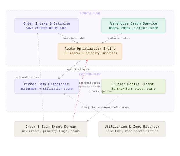
Architecture overview showing the order intake and batching service, warehouse graph service, route optimization engine, picker task dispatcher, event stream, and picker mobile client

The Order Intake and Batching Service is where individual orders stop being individual: it groups incoming orders into picker-sized batches, clustering by which pick zones their items touch so a single trip does not require crossing the whole facility. The Warehouse Graph Service owns the physical model of the building: aisles, cross-aisles, pick faces, and staging areas as a graph, with a precomputed distance cache so a “how far apart are these two points” query never requires a live pathfinding search. The Route Optimization Engine takes a batch and the distance cache and produces a near-optimal walking sequence using a TSP approximation, and it is also where a priority order gets stitched into an already-in-progress picker’s remaining stops. The Picker Task Dispatcher decides which idle or soon-to-be-idle picker receives a given computed route, balancing proximity against fairness so work does not pile up on the pickers closest to the loading dock. The Order and Scan Event Stream is the backbone that carries new orders, priority flags, and scan confirmations between every other component without anyone polling. The Picker Mobile Client is the handheld or wearable that renders the turn-by-turn stop list and reports scans back into the stream.

A batch’s life looks like this: orders land in the intake service and sit in a short queue until a wave closes, either because a timer expires or the batch hits capacity. The closed batch, along with the relevant slice of the distance cache from the Warehouse Graph Service, goes to the Route Optimization Engine, which returns a sequenced stop list within its latency budget. The Picker Task Dispatcher matches that route to a picker and pushes it to their mobile client. As the picker scans items, those confirmations flow back through the event stream, and if a new order arrives that plausibly fits inside that picker’s remaining walk, the event stream triggers the Route Optimization Engine’s fast insertion path instead of a full re-solve, and the updated route lands on the same picker’s handheld before they reach their next stop.

Key Insight

The single most important architectural decision is splitting route computation into two distinct algorithms with two distinct cost profiles: an expensive “build a route from scratch” path used only when a batch first forms, and a cheap “insert one stop into an already-committed route” path used for every subsequent priority order or dynamic addition. Trying to use one algorithm for both jobs either makes new-batch computation too slow or makes every mid-walk update disruptive enough to undo the picker’s progress.

Component Deep Dives

The Order Intake and Batching Wave

This component’s job is to decide which orders travel together in the same picker trip before any route is ever computed.

The obvious mistake is treating batching as an afterthought, batching orders strictly in arrival order until a cart is full. That produces batches whose items are scattered uniformly across the facility, and no amount of clever sequencing afterward can fix a batch that was doomed at formation, since a TSP solver can only optimize the order you visit stops in, not shrink how far apart those stops physically are. We batch by grouping orders whose items share zone footprint, using something close to a similarity clustering: two orders that both need items from zones 4 and 7 are strong candidates to travel together, while an order needing only zone 19 items is a weak fit for that same batch.

Orders arrive continuously, so batches form on a rolling wave: every 90 seconds, or sooner if a batch reaches its capacity limit (typically 12 to 20 stops per cart), the intake service closes whatever batch it has been assembling and hands it off. A wave timer that never closes would let pickers sit idle waiting for a “perfect” batch that never arrives during a slow period; a wave that closes too eagerly forfeits locality gains during a busy period when a slightly longer wait would have produced a much tighter batch.

# Wave-based order batching by zone-footprint similarity
# Demonstrates: greedy clustering of pending orders into capacity-bound batches
from dataclasses import dataclass, field
from time import monotonic

WAVE_INTERVAL_SECONDS = 90
MAX_BATCH_CAPACITY = 18          # stops a single cart/tote can carry
MIN_ZONE_OVERLAP = 0.35          # Jaccard similarity threshold to join a batch

@dataclass
class PendingOrder:
    order_id: str
    zones: set[str]
    item_count: int
    queued_at: float = field(default_factory=monotonic)

def zone_similarity(a: set[str], b: set[str]) -> float:
    if not a or not b:
        return 0.0
    return len(a & b) / len(a | b)

def form_batches(pending_orders: list[PendingOrder]) -> list[list[PendingOrder]]:
    # Oldest orders seed batches first, so nothing waits past the wave deadline.
    remaining = sorted(pending_orders, key=lambda o: o.queued_at)
    batches: list[list[PendingOrder]] = []

    while remaining:
        seed = remaining.pop(0)
        batch = [seed]
        batch_zones = set(seed.zones)
        stops_used = 1

        candidates = sorted(
            remaining,
            key=lambda o: zone_similarity(batch_zones, o.zones),
            reverse=True,
        )
        for candidate in candidates:
            if stops_used >= MAX_BATCH_CAPACITY:
                break
            if zone_similarity(batch_zones, candidate.zones) < MIN_ZONE_OVERLAP:
                continue
            batch.append(candidate)
            batch_zones |= candidate.zones
            stops_used += 1
            remaining.remove(candidate)

        batches.append(batch)

    return batches

Think of this like a shuttle van dispatcher deciding which airport passengers ride together, grouping people whose neighborhoods overlap rather than filling seats strictly in check-in order. What breaks if you skip zone clustering: a batch of 18 orders whose items are spread evenly across all 40 zones gives the Route Optimization Engine nothing to work with, since visiting 18 stops that are all roughly equidistant from each other has no meaningfully “better” order, and the picker ends up walking close to the worst-case distance no matter how the TSP solver sequences the stops.

Real World

This is the same instinct behind ride-share pooling algorithms like Uber Pool and Lyft Line: the hard problem is not routing two riders who are already in the same car, it is deciding which two riders should ever be matched into the same car in the first place. Warehouse batching and rideshare pooling both trade a slightly more complex matching step for a dramatically better routing problem downstream.

The Warehouse Graph Service

This component’s job is to turn the physical layout of the building into a graph that can answer “how far apart are any two points” fast enough to be called hundreds of times a minute.

The warehouse is modeled as a graph where nodes are aisle intersections, pick faces, staging lanes, and pack stations, and edges are the walkable segments between them, weighted by walking distance or time. Some edges are directional, since one-way aisles and forklift-restricted zones exist for pedestrian safety, and the graph must respect those constraints rather than assuming every edge is bidirectional.

At roughly 18,000 nodes, running a fresh shortest-path search for every pair of stops in every batch is too slow to hit a 300ms latency budget hundreds of times a minute. A full all-pairs distance table would need on the order of 18,000 squared entries, well over 300 million, which is wasteful to store and mostly irrelevant, since most pairs of nodes are never both stops in the same batch. Instead we precompute distances between a much smaller set of zone portal nodes, the entrances and exits of each of the 40 zones, and cache a local distance matrix inside each zone separately. A cross-zone distance becomes local-node-to-portal, plus portal-to-portal, plus portal-to-local-node, which collapses an 18,000-node shortest-path problem into a lookup against a few hundred precomputed portal distances and a small in-zone matrix.

# Zone-portal distance precomputation
# Demonstrates: reducing an 18,000-node facility graph to a small portal
# graph plus per-zone local matrices, refreshed incrementally on edge changes
import heapq
from collections import defaultdict

def dijkstra(graph: dict[str, list[tuple[str, float]]], source: str) -> dict[str, float]:
    distances = {source: 0.0}
    visited = set()
    heap = [(0.0, source)]
    while heap:
        dist, node = heapq.heappop(heap)
        if node in visited:
            continue
        visited.add(node)
        for neighbor, weight in graph.get(node, []):
            new_dist = dist + weight
            if new_dist < distances.get(neighbor, float("inf")):
                distances[neighbor] = new_dist
                heapq.heappush(heap, (new_dist, neighbor))
    return distances

def build_portal_matrix(graph: dict[str, list[tuple[str, float]]], portal_nodes: list[str]) -> dict[str, dict[str, float]]:
    # O(portals * (E log V)) - run once per graph rebuild, cached until the next one
    portal_matrix: dict[str, dict[str, float]] = {}
    for portal in portal_nodes:
        all_distances = dijkstra(graph, portal)
        portal_matrix[portal] = {p: all_distances[p] for p in portal_nodes if p in all_distances}
    return portal_matrix

def cross_zone_distance(
    local_to_portal: dict[str, float],
    portal_matrix: dict[str, dict[str, float]],
    portal_to_local: dict[str, float],
    origin_portal: str,
    dest_portal: str,
) -> float:
    return (
        local_to_portal[origin_portal]
        + portal_matrix[origin_portal][dest_portal]
        + portal_to_local[dest_portal]
    )

This is the same trick a road-trip GPS uses: it does not recompute a shortest path across an entire country’s road network every time you ask for directions, it leans on precomputed distances between major highway junctions and only runs a local search near your exact start and end points. What breaks without it: a single edge closure (an aisle blocked for a restock cart) would otherwise force a full graph-wide recomputation, when in reality only the local matrix for the affected zone, and the portal distances that route through it, need to be invalidated and rebuilt.

Real World

This is a lighter-weight version of contraction hierarchies, the technique behind fast road-network routers like OSRM: precompute shortcuts through a small set of “important” nodes so most queries only need a cheap lookup plus a small local search, instead of running full-graph Dijkstra on every request.

Watch Out

A common mistake is treating the graph as static once built. Aisle closures, spill cleanups, and temporary equipment blockages happen constantly on a warehouse floor, and a distance cache that only refreshes on the weekly slotting cycle will confidently route pickers through aisles that are not currently walkable. Edge-weight overrides for temporary closures need their own fast, incremental invalidation path, separate from the full offline graph rebuild.

The Route Optimization Engine

This component’s job is to take a batch’s stops and the distance cache and produce a near-optimal visiting order in well under 300ms, and to insert an urgent stop into an already-in-progress route even faster than that.

Internals of the Route Optimization Engine showing the nearest-neighbor construction, 2-opt local search loop with a time budget guard, and the separate cheapest-insertion path used for priority order injection

A smart engineer’s first instinct is to reach for an exact solver, since a batch of 15 to 20 stops sounds small enough to brute-force. It is not: the number of possible visiting orders for n stops is roughly n-factorial divided by two, and at 18 stops that is already in the trillions, far beyond anything an exact solver can chew through in a few hundred milliseconds, over and over, for hundreds of batches an hour. This is the traveling salesman problem, and it is NP-hard, which means we approximate rather than solve it exactly.

We build an initial tour with a greedy nearest-neighbor construction, always stepping to the closest unvisited stop, which runs in O(n^2) time and typically lands 20 to 25% above the true optimal distance. We then improve that tour with 2-opt local search: repeatedly look for two edges in the tour that, if swapped, shorten the total walk, and keep swapping until no improving swap exists or a time budget runs out. Because a batch’s stop count is bounded (12 to 20 stops), each 2-opt pass is cheap, and in practice a handful of milliseconds of 2-opt improvement brings the tour from roughly 20% above optimal down to 5 to 8% above optimal, comfortably inside the accuracy target.

A picker’s walk is not a closed loop back to where they started, it is a path from a fixed starting point (wherever their cart currently is) toward a pack station, so the algorithm anchors the first stop and, where relevant, the last stop, and only optimizes the order of everything in between.

# Nearest-neighbor construction + time-bounded 2-opt improvement
# Demonstrates: TSP-path approximation with a fixed start point and a
# hard time budget so the optimizer never blows the 300ms latency SLA
import time

def build_initial_tour(start: str, stops: list[str], dist) -> list[str]:
    unvisited = set(stops)
    tour = [start]
    current = start
    while unvisited:
        nxt = min(unvisited, key=lambda s: dist(current, s))
        tour.append(nxt)
        unvisited.remove(nxt)
        current = nxt
    return tour

def tour_length(tour: list[str], dist) -> float:
    return sum(dist(tour[i], tour[i + 1]) for i in range(len(tour) - 1))

def two_opt_improve(tour: list[str], dist, time_budget_seconds: float = 0.08) -> list[str]:
    deadline = time.monotonic() + time_budget_seconds
    improved = True
    best = tour[:]
    while improved and time.monotonic() < deadline:
        improved = False
        n = len(best)
        for i in range(1, n - 2):
            if time.monotonic() >= deadline:
                break
            for j in range(i + 1, n - 1):
                a, b, c, d = best[i - 1], best[i], best[j], best[j + 1]
                current_cost = dist(a, b) + dist(c, d)
                swapped_cost = dist(a, c) + dist(b, d)
                if swapped_cost < current_cost - 1e-9:
                    best[i:j + 1] = reversed(best[i:j + 1])
                    improved = True
    return best

def solve_batch_route(start: str, stops: list[str], dist, time_budget_seconds: float = 0.08) -> list[str]:
    initial = build_initial_tour(start, stops, dist)
    return two_opt_improve(initial, dist, time_budget_seconds)

Injecting a priority order into a route that is already in progress is a different problem with a different cost budget, and running the full nearest-neighbor-plus-2-opt pipeline on it would be both too slow and too disruptive, since it could reorder stops the picker has already effectively passed. Instead we use cheapest insertion: for the new stop, check every adjacent pair of remaining stops in the picker’s current route and find the single position where inserting it adds the least extra walking distance, then splice it in there, leaving every already-committed stop’s relative order untouched.

# Cheapest-insertion for priority order injection into an in-progress route
# Demonstrates: O(k) insertion against only the picker's *remaining* stops,
# never touching stops already visited or already committed ahead of them
def cheapest_insertion(remaining_route: list[str], new_stop: str, dist) -> tuple[list[str], float]:
    best_position = None
    best_added_cost = float("inf")

    for i in range(len(remaining_route) - 1):
        a, b = remaining_route[i], remaining_route[i + 1]
        added_cost = dist(a, new_stop) + dist(new_stop, b) - dist(a, b)
        if added_cost < best_added_cost:
            best_added_cost = added_cost
            best_position = i + 1

    new_route = remaining_route[:best_position] + [new_stop] + remaining_route[best_position:]
    return new_route, best_added_cost
Key Insight

The property that makes 2-opt work at this scale is that batch sizes are bounded by cart capacity, so every improvement pass stays cheap regardless of how large the facility grows. The property that makes cheapest insertion work for real-time re-routing is the opposite: it only ever considers the picker’s remaining, not-yet-visited stops, running in O(k) against a small k instead of re-running the full O(n^2) pipeline against the whole batch.

Watch Out

Re-running the full nearest-neighbor-plus-2-opt solve on every single new order arrival is a common shortcut that looks correct and performs badly in production. It is slow enough to blow the re-routing latency budget under load, and worse, a fresh solve has no memory of which stops the picker has already passed, so it can silently reorder the walk in a way that sends the picker backward through aisles they already cleared.

Zone-Based Picking and Cross-Zone Consolidation

This component’s job is to keep any single picker’s walking distance bounded regardless of how large the facility grows, by never asking one person to cross the entire floor for a single order.

An order whose ten items live in three zones that are, say, a third of a mile apart from each other is a bad candidate for a single picker’s single trip, even with a perfect TSP solve, because the TSP solver can only optimize the order stops are visited in, not shrink the underlying distances between them. Zone-based picking splits such an order into per-zone sub-picks: one picker working zone 4 grabs that zone’s items, a different picker working zone 19 grabs theirs, and both sub-picks converge at a shared consolidation point before the order moves on to packing.

This is the same idea as a relay race: each runner covers one leg of the course and hands off a baton at a checkpoint, rather than one runner attempting the entire distance alone. The tradeoff is real: consolidation adds a coordination step and a small amount of extra handling per multi-zone order, since two separate pick events now have to be reconciled into one shipment. But it bounds the worst case, so a facility can grow from 500,000 to 1,000,000 square feet without any single picker’s maximum possible walk growing along with it.

Key Insight

The property that keeps the 300ms latency target achievable as the facility grows is that zone-based picking shrinks the routing problem’s scope along with it. Route computation happens against a roughly 400-to-500-node zone subgraph, not the full 18,000-node facility graph, so adding more zones adds more parallel, independently-sized routing problems rather than one larger one.

Picker Task Dispatcher and Utilization Balancing

This component’s job is to decide which idle or soon-to-be-idle picker gets a given computed route, balancing distance against fairness so work does not pile up on whichever picker happens to be standing closest to the queue.

The obvious approach, always assigning a batch to whichever idle picker is physically nearest its first stop, minimizes deadhead walking in the short term but starves pickers working in the facility’s less-trafficked corners, since batches near the busy zones keep getting formed and assigned faster than batches near the quiet ones. Over a nine-hour shift that produces a wide utilization gap: some pickers finish far more batches than others despite putting in the same hours, which is both an efficiency loss (idle labor) and a fairness problem.

We score each idle picker against each pending route using a weighted combination of distance, zone specialization, and a utilization term that favors pickers who have been idle longest or completed fewer batches so far in the shift.

# Picker-to-route assignment scoring
# Demonstrates: balancing proximity against fairness so utilization
# does not concentrate on pickers nearest the busiest zones
from dataclasses import dataclass

DISTANCE_WEIGHT = 0.5
ZONE_MATCH_WEIGHT = 0.2
UTILIZATION_WEIGHT = 0.3

@dataclass
class Picker:
    picker_id: str
    current_node: str
    zone_specialization: str | None
    idle_seconds: float
    batches_completed_this_shift: int

@dataclass
class PendingRoute:
    batch_id: str
    first_stop: str
    primary_zone: str

def assignment_score(picker: Picker, route: PendingRoute, dist, max_idle_seconds: float, max_batches: int) -> float:
    distance_term = 1.0 - min(dist(picker.current_node, route.first_stop) / 500.0, 1.0)
    zone_term = 1.0 if picker.zone_specialization == route.primary_zone else 0.0
    idle_term = picker.idle_seconds / max(max_idle_seconds, 1.0)
    load_term = 1.0 - (picker.batches_completed_this_shift / max(max_batches, 1))
    utilization_term = (idle_term + load_term) / 2.0

    return (
        DISTANCE_WEIGHT * distance_term
        + ZONE_MATCH_WEIGHT * zone_term
        + UTILIZATION_WEIGHT * utilization_term
    )

def assign_route(idle_pickers: list[Picker], route: PendingRoute, dist) -> Picker:
    max_idle = max((p.idle_seconds for p in idle_pickers), default=1.0)
    max_batches = max((p.batches_completed_this_shift for p in idle_pickers), default=1)
    return max(
        idle_pickers,
        key=lambda p: assignment_score(p, route, dist, max_idle, max_batches),
    )

The analogy here is a taxi dispatcher balancing “send the nearest driver” against “send the driver who has been waiting longest without a fare,” so income and workload spread across the fleet instead of concentrating on drivers parked next to the busiest pickup spot. What breaks without the utilization term: pickers assigned to quiet zones effectively get penalized for their location, finishing fewer batches per shift through no fault of their own, which shows up later as an uneven labor cost and a morale problem, not just a routing inefficiency.

Real World

UPS’s ORION system, one of the most cited real-world deployments of route optimization at scale, blends exactly this kind of multi-factor scoring for its delivery drivers, weighing distance savings against operational constraints rather than optimizing distance alone, and reports saving on the order of 100 million miles driven per year across its fleet from smarter sequencing.

The Order and Scan Event Stream and Dynamic Re-Routing

This component’s job is to get new orders, priority flags, and scan confirmations to the components that need them within the latency budget, without anyone polling for updates.

New orders, rush flags, and scan events all publish onto a small set of topics, and both the Route Optimization Engine and Picker Task Dispatcher consume from them. When a new order arrives, the stream’s consumer checks eligibility before doing anything expensive: is there an active picker whose remaining stops pass near this order’s zone within an acceptable detour threshold? If yes, the cheapest-insertion path runs and the picker’s route updates in place. If no picker is a good fit, the order falls back to the next batching wave instead of forcing a route to accept a bad detour just because it happened to arrive at the wrong moment.

// Priority order eligibility check and re-route trigger
// Demonstrates: deciding whether a new order can be cheaply inserted into
// an in-progress picker's route, anchored to their real-time position
package rerouting

import (
	"context"
	"time"
)

type Picker struct {
	ID              string
	CurrentNode     string
	RemainingStops  []string
	LastScanAt      time.Time
}

type NewOrderEvent struct {
	OrderID     string
	PrimaryZone string
	PickupNode  string
	Priority    bool
}

const maxDetourMeters = 120.0
const stalePositionThreshold = 45 * time.Second

func (s *ReroutingService) HandleNewOrder(ctx context.Context, evt NewOrderEvent) error {
	candidates := s.activePickersNear(evt.PrimaryZone)

	for _, picker := range candidates {
		// A picker whose last scan is stale might already be past the point
		// our route model thinks they are, so we skip rather than guess.
		if time.Since(picker.LastScanAt) > stalePositionThreshold {
			continue
		}

		route, addedDistance := cheapestInsertion(picker.RemainingStops, evt.PickupNode, s.distance)
		if addedDistance > maxDetourMeters && !evt.Priority {
			continue
		}

		if err := s.pushRouteUpdate(ctx, picker.ID, route); err != nil {
			return err
		}
		return s.markOrderAssigned(ctx, evt.OrderID, picker.ID)
	}

	// No in-progress picker is a good fit; the order waits for the next wave.
	return s.returnToBatchQueue(ctx, evt.OrderID)
}

The analogy is an air traffic controller radioing a small course correction to a plane already in the air, rather than grounding the flight and replanning its whole itinerary from the gate. A rush order, marked Priority: true, is allowed to exceed the normal detour threshold, since the cost of a slightly longer walk is smaller than the cost of missing the truck it needs to catch.

Watch Out

A common mistake is anchoring the insertion candidates to the batch’s original stop list order instead of the picker’s actual, current position. Scan events are the only reliable signal for where a picker really is; a route model that trusts the plan instead of the picker’s last confirmed scan can insert a new stop into a spot the picker has functionally already walked past, forcing an unnecessary backtrack. Treating a stale last-scan timestamp as a reason to skip that picker for injection, as the code above does, avoids exactly that failure.

Data Model

The data model spans five entities: orders and their items, batches and their sequenced stops, the warehouse graph’s static topology, pickers and their live state, and pick events for auditing and exception handling.

-- Orders and order items: the unit of customer-facing work
CREATE TABLE orders (
    order_id        BIGINT      PRIMARY KEY,
    placed_at       TIMESTAMPTZ NOT NULL DEFAULT NOW(),
    priority        BOOLEAN     NOT NULL DEFAULT FALSE,
    status          TEXT        NOT NULL DEFAULT 'pending'
        CHECK (status IN ('pending', 'batched', 'picking', 'picked', 'exception', 'shipped')),
    ship_by         TIMESTAMPTZ NOT NULL
);

CREATE TABLE order_items (
    id              BIGSERIAL   PRIMARY KEY,
    order_id        BIGINT      NOT NULL REFERENCES orders(order_id),
    sku             TEXT        NOT NULL,
    bin_location    TEXT        NOT NULL,     -- references warehouse_nodes.node_id
    zone_id         TEXT        NOT NULL,
    quantity        INT         NOT NULL CHECK (quantity > 0),
    picked_at       TIMESTAMPTZ
);

CREATE INDEX ON order_items (order_id);
CREATE INDEX ON order_items (zone_id);

-- Batches: the picker-facing unit of work, one sequenced route per batch
CREATE TABLE batches (
    batch_id            BIGSERIAL   PRIMARY KEY,
    formed_at           TIMESTAMPTZ NOT NULL DEFAULT NOW(),
    picker_id           TEXT        REFERENCES pickers(picker_id),
    status              TEXT        NOT NULL DEFAULT 'routed'
        CHECK (status IN ('routed', 'in_progress', 'completed', 'exception')),
    primary_zone        TEXT        NOT NULL,
    route_computed_ms   INT         NOT NULL,   -- optimizer latency, tracked for SLA monitoring
    route_quality_ratio NUMERIC(4,3)            -- computed distance / lower-bound estimate
);

CREATE TABLE batch_stops (
    id              BIGSERIAL   PRIMARY KEY,
    batch_id        BIGINT      NOT NULL REFERENCES batches(batch_id),
    order_id        BIGINT      NOT NULL REFERENCES orders(order_id),
    node_id         TEXT        NOT NULL,
    sequence_index  INT         NOT NULL,
    inserted_via    TEXT        NOT NULL DEFAULT 'initial_solve'
        CHECK (inserted_via IN ('initial_solve', 'cheapest_insertion')),
    completed_at    TIMESTAMPTZ
);

CREATE UNIQUE INDEX ON batch_stops (batch_id, sequence_index);
CREATE INDEX ON batch_stops (batch_id) WHERE completed_at IS NULL;

-- Warehouse graph: static topology plus dynamic edge overrides
CREATE TABLE warehouse_nodes (
    node_id     TEXT PRIMARY KEY,
    zone_id     TEXT NOT NULL,
    node_type   TEXT NOT NULL CHECK (node_type IN ('intersection', 'pick_face', 'staging', 'pack_station', 'portal')),
    x_coord     NUMERIC NOT NULL,
    y_coord     NUMERIC NOT NULL
);

CREATE TABLE warehouse_edges (
    id              BIGSERIAL PRIMARY KEY,
    from_node       TEXT NOT NULL REFERENCES warehouse_nodes(node_id),
    to_node         TEXT NOT NULL REFERENCES warehouse_nodes(node_id),
    base_weight     NUMERIC NOT NULL,       -- steady-state walking distance/time
    directional     BOOLEAN NOT NULL DEFAULT FALSE,
    override_weight NUMERIC,                -- NULL unless temporarily closed/slowed
    override_until  TIMESTAMPTZ
);

CREATE INDEX ON warehouse_edges (from_node);
CREATE INDEX ON warehouse_edges (to_node) WHERE directional = FALSE;

-- Pickers: live operational state, read on every assignment and re-route decision
CREATE TABLE pickers (
    picker_id                  TEXT PRIMARY KEY,
    current_node               TEXT NOT NULL REFERENCES warehouse_nodes(node_id),
    zone_specialization        TEXT,
    shift_started_at           TIMESTAMPTZ NOT NULL,
    idle_since                 TIMESTAMPTZ,
    batches_completed_shift    INT NOT NULL DEFAULT 0,
    last_scan_at               TIMESTAMPTZ
);

-- Pick events: append-only, backs both progress tracking and exception analysis
CREATE TABLE pick_events (
    id              BIGSERIAL   PRIMARY KEY,
    batch_id        BIGINT      NOT NULL REFERENCES batches(batch_id),
    order_id        BIGINT      NOT NULL,
    node_id         TEXT        NOT NULL,
    event_type      TEXT        NOT NULL CHECK (event_type IN ('scan', 'short_pick', 'substitution')),
    occurred_at     TIMESTAMPTZ NOT NULL DEFAULT NOW()
);

CREATE INDEX ON pick_events (batch_id, occurred_at);
CREATE INDEX ON pick_events (event_type, occurred_at DESC) WHERE event_type != 'scan';

warehouse_edges is where the incremental invalidation from the Warehouse Graph Service actually lives: an aisle closure is a row-level override_weight and override_until update, not a rebuild of the whole graph, which is what keeps a temporary blockage propagating within the 60-second freshness target. pickers.current_node and last_scan_at are the two columns the dynamic re-routing path reads on every eligibility check, so they are kept in a small, hot, frequently-updated table separate from the larger historical pick_events log.

Data flow diagram showing an order's lifecycle from placement through batch formation, route publication, active picking with possible priority injection, and completion or exception handling

An order is born pending, moves to batched the moment a wave closes around it, and to picking once its batch is assigned and a picker starts walking. Its individual order_items rows fill in picked_at as scans come in. If every item in an order scans successfully, the order moves to picked and eventually shipped; if any item comes up short, a pick_events row with event_type = 'short_pick' is written and the order can move to exception for a substitution or backorder decision, shown as its own terminal path in the data flow diagram above.

Key Insight

Sharding pick_events or batch_stops by picker_id would optimize for “show me one picker’s history,” but the actual hot query pattern during a shift is “what does this specific batch’s remaining route look like right now,” a query scoped by batch_id, not picker_id. Indexing and partitioning around batch_id and recency, rather than picker identity, keeps the dominant read path fast.

Key Algorithms and Protocols

Nearest-Neighbor Construction and 2-opt Improvement

Covered in the Route Optimization Engine section above, this pair of algorithms is the core of batch route computation: a greedy O(n^2) construction followed by a time-bounded O(n^2) per-pass local search that stops the moment no improving swap exists or the time budget runs out.

Key Insight

The property that makes this pair reliable rather than merely fast is that 2-opt can only ever improve or match the nearest-neighbor tour it starts from, never make it worse, since it only accepts a swap when the resulting tour is strictly shorter. Bounding it with a wall-clock deadline instead of an iteration count means the algorithm’s latency stays predictable even if a particular batch’s geometry happens to need more improving passes than usual.

Cheapest Insertion for Priority Injection

Covered in the Route Optimization Engine section above, cheapest insertion runs in O(k) against only a picker’s remaining, not-yet-visited stops, checking every adjacent pair for the least-cost place to splice in one new stop.

Key Insight

The property that makes this safe to run inline, synchronously, as events arrive is that it never touches stops before the insertion point, so a picker’s already-committed path never gets reshuffled underneath them. A full TSP re-solve does not have this property, which is exactly why it is the wrong tool for a live re-route.

Zone-Portal Distance Precomputation

Covered in the Warehouse Graph Service section above, this algorithm reduces an all-pairs shortest-path problem across roughly 18,000 nodes down to Dijkstra runs from a much smaller set of portal nodes, each in O(E log V) time, cached until the next incremental edge update invalidates the affected region.

Key Insight

The property that makes this scale as the facility grows is that the portal graph’s size is governed by the number of zones, not the number of bin locations. Adding more pick faces inside an existing zone does not grow the portal matrix at all; it only grows the small in-zone local matrix for that one zone.

Zone-Footprint Similarity Batching

Covered in the Order Intake and Batching Wave section above, batch formation scores candidate orders by Jaccard similarity between their zone sets, a simple set-intersection-over-union computation that runs in time proportional to the number of zones an order touches, negligible against typical order sizes.

Key Insight

The property that makes this batching heuristic effective is that it optimizes for the thing the TSP solver cannot fix afterward: physical proximity between stops. A better sequencing algorithm downstream can never compensate for a batch whose items were never close together to begin with.

Scaling and Performance

The Route Optimization Engine and the Warehouse Graph Service’s distance cache are the two components under the most sustained load, and they scale differently: the optimizer is a stateless, per-batch compute job that scales horizontally behind a worker pool, while the distance cache is read-heavy and scales by sharding along the same zone boundaries the rest of the system already uses for batching and picking.

Scaling diagram showing zone-sharded route optimizer worker pools, a cross-zone coordinator for multi-zone orders, and a replicated distance cache fed by the offline facility graph rebuild
Capacity Estimation:

Given:
  - 1,000,000 sq ft facility, ~40 pick zones, ~18,000 graph nodes
  - Peak order rate: 50,000 orders/hour (~14/sec)
  - Average batch size: 12 orders/batch
  - Route compute time budget: 300ms p99, ~80ms actual 2-opt budget

Batch formation rate at peak:
  14 orders/sec / 12 orders per batch = ~1.2 batches/sec formed

Route Optimization Engine worker sizing:
  1.2 batches/sec * ~80ms compute time = ~0.1 CPU-seconds/sec of steady load
  Provisioning 8-10 workers per zone-shard group gives 60-80x headroom
  for compute-time variance and simultaneous priority re-route requests.

Distance cache size (portal-reduced):
  ~40 zones => ~200-400 portal nodes total (5-10 portals per zone)
  Portal matrix: 400^2 * 8 bytes (float64) = ~1.3 MB, trivially cached in memory
  Per-zone local matrix: ~450 nodes/zone => 450^2 * 8 bytes = ~1.6 MB/zone
  40 zones * 1.6 MB = ~64 MB total local matrices, comfortably fits in a
  single cache node per facility, replicated per zone-shard for locality.

Event stream throughput:
  50,000 orders/hour * ~12 items/order average = 600,000 scan events/hour
  = ~167 scan events/sec at peak, each a small (<1 KB) message - a light
  load for any commodity pub/sub system.

Picker fleet sizing:
  500 pickers/shift, ~12-minute average batch walk time =>
  500 pickers * (60 min / 12 min per batch) = ~2,500 batches/hour capacity
  against a ~1,250 batches/hour peak demand (50,000 orders / 40 order-equivalent
  batches), leaving headroom for batches with above-average walk time.

The dominant bottleneck is not the optimizer’s raw compute, it is keeping the distance cache both fast and fresh: a stale cache after an aisle closure produces routes through aisles that are not actually walkable, while a cache that recomputes too eagerly wastes CPU on zones nothing has changed in. Sharding the cache and the optimizer worker pools along zone boundaries, the same boundaries batching and picking already use, means a facility can add zones without any single shard’s load growing, and a Cross-Zone Coordinator only gets involved for the minority of orders that genuinely span zones far enough apart to need splitting.

Real World

Amazon’s fulfillment centers are widely reported to combine zone-based picking with algorithmic batching for exactly this reason: a facility can grow well past a million square feet without any individual picker’s maximum walk distance growing proportionally, because the routing problem is deliberately kept zone-scoped rather than solved as one giant facility-wide TSP.

Failure Modes and Recovery

FailureDetectionImpactRecovery
Warehouse graph edge closure not propagatedPicker reports blocked aisle via handheld, or repeated route-abandonment events from one nodePickers routed through a physically blocked path, wasted walk and backtrackManual override endpoint sets override_weight immediately; incremental invalidation rebuilds only the affected zone’s local matrix, not the whole graph
Route Optimization Engine overloaded or timing outp99 latency alarm on route computation, worker queue depth growingNew batches wait longer than the 300ms target, pickers may go briefly idleAutoscale the worker pool per zone-shard; fall back to plain nearest-neighbor (skip 2-opt) under sustained overload rather than missing the latency SLA entirely
Picker Task Dispatcher assigns a batch to a picker who went on breakHandheld heartbeat missing, or no scan activity within expected time after assignmentAssigned batch sits un-started, order ship-by deadline at riskDispatcher requires a recent heartbeat before assignment; a batch with no pick activity within a threshold is automatically reassigned to another idle picker
Event stream lag causes duplicate or late priority injectionConsumer lag metric on the priority-order topic exceeds thresholdA rush order’s re-route lands after the picker has already passed the best insertion pointCheapest insertion is idempotent per order_id; a late-arriving injection re-evaluates against the picker’s current remaining stops rather than blindly applying a stale plan
Distance cache corruption or bad rebuildRoute quality ratio (computed distance vs. lower-bound estimate) spikes across many batches at onceRoutes still compute, but walking distances balloon fleet-wideServe the previous known-good cache generation while a fresh rebuild runs; alert if route_quality_ratio crosses a threshold, since it is a fast fleet-wide signal that something upstream is wrong
Picker handheld goes offline mid-batchMissing heartbeat and no scans from that device for several minutesThat picker’s in-progress batch stalls, priority injection cannot reach themDispatcher marks the picker unavailable after a timeout, requeues incomplete stops into the next wave for a different picker, and flags the partial batch for manual reconciliation
Watch Out

The most common operational mistake is assuming that because routes are computed algorithmically, a bad route will always be obviously bad and get caught immediately. In practice a subtly stale distance cache or a slightly wrong zone boundary produces routes that are only 15 to 20% worse than they should be, easy to miss shift over shift, and it compounds into a real productivity loss before anyone notices, since no single route looks broken enough to trigger a complaint.

Comparison of Approaches

ApproachLatency per batchComplexityFailure modeBest fit
FIFO single-order picking, no batchingInstant (no computation)Very lowLabor cost scales linearly with order count regardless of layoutVery small facilities or extremely low order volume
Batching + nearest-neighbor only, no 2-optSub-10msLowRoutes land 20-25% above optimal, leaving real distance savings on the tableEarly-stage systems prioritizing simplicity over route quality
Batching + nearest-neighbor + 2-opt (this design)Tens of milliseconds, bounded by time budgetMedium-highRequires a bounded time budget and careful edge-case handling for fixed start/end pointsLarge facilities (500,000+ sq ft) needing both speed and route quality
Exact TSP solve (branch-and-bound / ILP)Seconds to minutes at 15+ stopsVery highComputation time explodes combinatorially past a dozen stops, unusable at this latency budgetSmall, fixed batch sizes where perfect optimality justifies heavy compute, rarely applicable at fulfillment-center scale
Fixed zone-pick-and-pass, no dynamic re-routingPrecomputed, effectively zero runtime costLowCannot absorb new or priority orders without waiting for the next full waveFacilities with highly predictable, low-variance order volume

We would pick batching combined with nearest-neighbor-plus-2-opt for any facility past a few hundred thousand square feet, because it is the only approach on this list that hits both the latency budget and a route quality close enough to optimal to matter economically. The alternatives fail on one axis each: no batching leaves throughput on the table regardless of routing quality, nearest-neighbor alone leaves 15-20% of achievable distance savings unclaimed, an exact solve is computationally out of reach at these batch sizes and call volumes, and a fixed pick-and-pass scheme cannot absorb the priority orders that, in practice, arrive continuously throughout a shift.

Key Takeaways

  • Order batching by zone-footprint similarity, not arrival order, is what makes the downstream routing problem solvable. No sequencing algorithm can fix a batch whose items were never physically close together.
  • The traveling salesman problem is NP-hard, so the system never attempts an exact solve. Nearest-neighbor construction followed by time-bounded 2-opt local search reliably lands within 5-8% of optimal in milliseconds.
  • Priority order injection uses a completely different algorithm, cheapest insertion, from initial route computation. Running the full TSP pipeline on every new order arrival is both too slow and disruptive to a picker’s already-committed progress.
  • The warehouse graph is reduced to a small portal network plus per-zone local matrices, so a distance lookup never requires a full-graph shortest-path search, and an aisle closure only invalidates the affected zone.
  • Zone-based picking bounds the worst case as the facility grows. Splitting multi-zone orders into per-zone sub-picks that converge at a consolidation point means no single picker’s maximum possible walk grows with total facility size.
  • Picker utilization balancing has to weigh fairness against proximity, or pickers working the facility’s quieter corners are systematically penalized by pure nearest-picker assignment.
  • Dynamic re-routing must anchor to a picker’s real, scan-confirmed position, not their planned position. A stale position estimate turns a helpful mid-walk insertion into an unnecessary backtrack.
  • Route quality ratio is a cheap, fleet-wide early warning signal. A spike in computed-versus-lower-bound distance across many batches at once usually means the distance cache or graph data is wrong, well before any single route looks obviously broken.

The counter-intuitive lesson is that the hardest-sounding part of this system, the TSP approximation itself, is actually the most standard and best-understood piece of the whole design. The parts that separate a working system from a merely functional one are upstream and downstream of the solver: batching orders so the solver has something worth optimizing, and injecting priority orders through a fundamentally different, cheaper algorithm so real-time updates never have to pay the cost of a full re-solve.

Frequently Asked Questions

Q: Why not just run an exact TSP solver for these routes, since batches are only 12 to 20 stops, which sounds small?

A: Twelve to twenty stops sounds small until you count the possible orderings: the number of distinct visiting sequences grows factorially, and at 18 stops that number is already in the trillions. An exact branch-and-bound or ILP solver can sometimes handle that in seconds to minutes for a single instance, but this system needs to solve well over a thousand such instances per hour, each within a 300ms budget, which rules out exact solving entirely. Nearest-neighbor plus time-bounded 2-opt trades a small, bounded amount of route quality for a predictable, sub-100ms compute cost.

Q: Why not just compute a fresh shortest path with Dijkstra every time you need a distance, instead of maintaining a precomputed distance cache?

A: At roughly 18,000 graph nodes, a fresh Dijkstra run for every pairwise distance a route computation needs would make the 300ms latency budget essentially impossible to hit under load, since a single batch can need dozens of pairwise distances and the system runs many batches every second. Precomputing a small portal-node matrix and per-zone local matrices turns most distance lookups into array reads instead of graph searches, at the cost of needing an incremental invalidation path when the graph changes.

Q: Why maintain a separate cheapest-insertion algorithm instead of just re-running the batch solver whenever a priority order needs to go in?

A: Re-running the full pipeline treats the picker’s remaining stops as an unordered set to be re-solved from scratch, which can silently reorder stops the picker has already effectively passed and takes an order of magnitude longer than a targeted insertion. Cheapest insertion only ever considers where to splice one new stop into the existing, already-committed sequence, so it preserves the picker’s progress and runs fast enough to execute synchronously as events arrive.

Q: How do you handle an order whose items are split across zones that are far apart, without forcing one picker to walk the entire facility?

A: That is exactly what zone-based picking and cross-zone consolidation exist for. Rather than routing one picker through every zone an order touches, the order is split into per-zone sub-picks, each handled by a picker already working that zone, and the pieces converge at a shared consolidation point before the order moves on. It costs a small amount of extra coordination per multi-zone order, but it keeps any individual picker’s walking distance bounded regardless of how spread out that particular order’s items happen to be.

Q: What stops the system from repeatedly assigning the best batches to the same handful of pickers near the busiest zones?

A: The Picker Task Dispatcher’s assignment score is not distance-only; it blends proximity with a utilization term that favors pickers who have been idle longer or completed fewer batches so far in the shift. A picker working a quieter corner of the facility is more likely to win the next assignment even if they are slightly farther from that batch’s first stop, which keeps completed-batch counts from diverging too far across the fleet over a full shift.

Q: What happens to route quality if the Route Optimization Engine falls behind and cannot run 2-opt within its time budget?

A: The system degrades gracefully rather than failing closed. If the 2-opt improvement loop cannot complete even one full pass before its deadline, the batch ships with the nearest-neighbor construction alone, which is roughly 20% above optimal instead of 5-8%, worse but still a valid, walkable route. That is a deliberate design choice: a picker with a slightly longer route is far better than a picker with no route at all while the optimizer catches up.

Interview Questions

Q: Walk through how you would compute a route for a newly formed batch of 15 orders, from the batch closing to the route landing on a picker’s handheld.

Expected depth: Cover pulling the relevant zone-portal and local distance data from the Warehouse Graph Service, building an initial tour with nearest-neighbor construction anchored to the picker’s actual starting position, improving it with time-bounded 2-opt, and handing the result to the Picker Task Dispatcher for assignment. Discuss why the algorithm treats this as a path problem with a fixed start (and often a fixed end at a pack station) rather than a closed-loop tour, and how the 300ms latency budget is split across these stages.

Q: A rush order arrives that needs to go out on the next truck. Design the decision logic for whether to inject it into an already-in-progress picker’s route versus letting it wait for the next batching wave.

Expected depth: Explain the eligibility check (is there an active picker whose remaining stops are near this order’s pickup zone), the cheapest-insertion cost calculation, and why a priority order is allowed a larger detour threshold than a normal one. Discuss the risk of anchoring the insertion to a stale position estimate instead of the picker’s most recent scan, and what happens if no picker is currently a good fit.

Q: How would you redesign the warehouse graph and distance cache if the facility doubled in size to 2,000,000 square feet without a proportional increase in route computation latency?

Expected depth: Discuss why the portal-node reduction scales with zone count rather than raw node count, how zone-based picking bounds any individual picker’s or any individual routing subproblem’s size, and how sharding both the distance cache and the Route Optimization Engine’s worker pools along zone boundaries lets the facility grow by adding more parallel shards rather than making any existing shard’s problem larger.

Q: A platform team notices that pickers in one corner of the warehouse are completing noticeably fewer batches per shift than everyone else, even though their walk times look normal. What would you check?

Expected depth: Point to the Picker Task Dispatcher’s assignment scoring as the likely culprit, specifically whether the utilization term is properly weighted against the distance term, or whether that corner’s zone is systematically underrepresented in batch formation due to low order density there. Discuss how to distinguish “this picker is assigned fewer batches” from “this zone simply generates fewer batches” using the batches_completed_shift and route_quality_ratio data already in the schema.

Q: What would you change about the batching wave if the facility needed to support same-hour rush fulfillment for a subset of orders, rather than the normal 90-second wave cadence?

Expected depth: Discuss shortening the wave interval or introducing a separate, faster wave tier for flagged rush orders, the tradeoff between wave latency and batch quality (a wave closed too early has less time to find zone-similar orders to cluster together), and why priority injection into already-in-progress routes, not just faster batch formation, is usually the better lever for genuinely urgent single orders that cannot wait even for a short wave.

Premium Content

Unlock the full article along with everything else in the archive — all in one place.

In-depth analysis Expert insights Full archive access
Unlock Full Article