Picture the host of a large industry conference who is genuinely good at introductions. She does not hand you a directory of every attendee, and she does not just introduce you to whoever happens to be standing closest. She thinks about who you already know, glances at who those people know, and introduces you to the handful of strangers you are two handshakes away from, favoring the ones several of your acquaintances already know well over the one your colleague met once at the bar. That is a second-degree introduction, and it works as a heuristic because a friend of a friend, especially one several friends have in common, is a far better bet than a total stranger picked at random.

Now replace the host with a recommendation engine, replace a room of a few hundred attendees with a social graph of 500 million nodes, and replace a handful of quiet introductions with a “who to follow” widget that has to compute a fresh short list for hundreds of millions of people every single day, without ever making a single user wait more than a few hundred milliseconds to see it. The engineering problem is exactly the one the host solves, but at a scale where “look at who your friends know” stops being a quick mental exercise and becomes a distributed traversal over tens of billions of edges, some of which belong to accounts so widely followed that expanding their neighbor list even once could touch millions of rows.

The naive approach, run a live breadth-first search over the follow graph the instant a user opens the app, fails for a boring but decisive reason: an ordinary account follows on the order of a hundred people, but the graph’s degree distribution is a power law, and a meaningful fraction of any user’s friend-of-friend walk passes through at least one hub account with an out-degree or in-degree in the millions. Expanding that one node fully turns a bounded, cheap traversal into an unbounded, slow one, and it happens often enough that “just run BFS on read” produces unpredictable, frequently unacceptable latency. The opposite naive approach, precompute nothing and always fall back to a simple popularity list, avoids the latency problem entirely but throws away the entire reason a graph-based recommendation is good in the first place: it stops being personalized to the one graph that is actually relevant, yours.

We need to solve for three things simultaneously: a traversal strategy that can walk two hops out from every one of 500 million users without letting a single hub account blow up the cost of that walk, a pruning and scoring pipeline that turns tens of thousands of raw second-degree candidates into a short, meaningfully ranked list cheaply enough to run for hundreds of millions of users a day, and a clean separation between the steady-state case, where a user already has an established graph and yesterday’s precomputed answer is good enough, and the cold-start case, where a brand-new account has no graph signal to traverse at all.

Requirements and Constraints

Functional Requirements

• Ingest follow and unfollow edges into a partitioned graph store as they happen, keeping both a forward adjacency (who I follow) and a reverse adjacency (who follows me) available for downstream use
• For every eligible user, traverse outward to second-degree connections, friends of friends, bounded by a fan-out cap, and produce a shortlist of candidates the user does not already follow
• Score each surviving candidate primarily by mutual connection count, blended with a decayed activity signal, so a candidate who shares ten mutual friends but has not logged in for a year does not automatically outrank one with six mutual friends who is active daily
• Prune candidates aggressively before scoring: exclude already-followed accounts, blocked or muted accounts, previously dismissed candidates, and anyone below a minimum mutual-connection threshold
• Recompute the full recommendation list for every eligible user on a daily cadence via an offline batch job, rather than on every read
• Serve a ranked “who to follow” list on demand from the precomputed output through a low-latency read path
• Handle new users who have too few, or zero, graph edges to produce a meaningful second-degree traversal, through a distinct cold-start strategy that does not depend on the batch job having ever run for them
• Let a user dismiss or hide a recommended candidate, and never resurface that exact candidate again for that user

Non-Functional Requirements

• Scale: 500 million total user nodes in the social graph, average out-degree (accounts followed) of roughly 120, producing around 60 billion directed follow edges stored forward, mirrored by a reverse index of comparable size
• Batch throughput: the nightly refresh covers roughly 220 million users who were active in the last 30 days, and the full run must complete inside a bounded nightly compute window, targeted at 4 hours
• Read latency: the “who to follow” widget’s precomputed read path targets a p99 under 150ms
• Cold-start latency: the on-demand fallback for a user with no batch-computed row must respond within roughly 300ms, since it is served synchronously on request rather than precomputed
• Freshness: a batch-computed recommendation list may lag the live graph by up to 24 hours; a follow made five minutes ago does not need to instantly change someone else’s recommendations, but a suppression, a user dismissing a candidate, must take effect immediately, not on the next nightly run
• Availability: the online read path targets 99.9% uptime; the graph write path (the follow/unfollow feature itself) must never be blocked, throttled, or slowed by the batch job’s read load against the same storage layer
• Bounded fan-out: no single user’s traversal may expand a hub node’s full neighbor list; fan-out per hop must stay bounded regardless of how large any individual node’s true degree is

Constraints and Assumptions

• Turn-by-turn UI rendering of the “who to follow” widget, push notifications, and any A/B experimentation framework around recommendation placement are out of scope; this design only decides who to suggest and in what order
• The follow/unfollow feature itself, meaning the write path that lets a user actually follow someone, is owned by a separate profile and graph-edge service; this design treats it as an upstream event stream, not something we build here
• We assume the graph is stored in a distributed, partitioned adjacency-list store, comparable to a wide-column store; we design its schema and partitioning key, not the storage engine itself
• We assume a separate content and interest classification service exists and can supply an interest-tag signal per user, used only by the cold-start fallback, never by the primary mutual-friend scoring path
• We treat account-level moderation (spam detection, ban lists) as an upstream signal this system consumes through the blocked and muted sets, not something it computes

High-Level Architecture

The system has five major components: the Graph Ingestion and Partitioned Storage Layer, the Bounded BFS Traversal Engine, the Candidate Pruning and Mutual-Connection Scorer, the Offline Batch Recommendation Pipeline, and the Online Serving Layer and Cold-Start Handler.

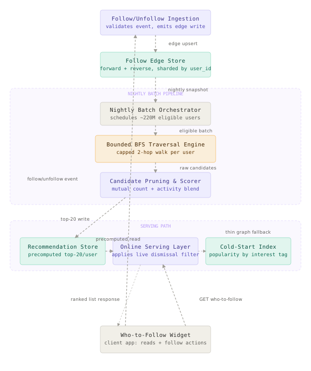
The Graph Ingestion and Partitioned Storage Layer is the front door for every follow and unfollow action: it validates the event and writes it into a sharded edge store that both the live write path and the nightly batch job can read without contention. The Bounded BFS Traversal Engine is the computational core, run once per eligible user per night, walking two hops out from that user’s own follows with a hard cap on how many edges it will expand at each hop. The Candidate Pruning and Mutual-Connection Scorer takes the raw, noisy set of second-degree candidates that traversal produces and turns it into a short, ranked list by excluding the obviously irrelevant candidates cheaply before spending anything on expensive per-candidate scoring. The Offline Batch Recommendation Pipeline is the orchestration layer that runs the traversal and scoring steps across the entire eligible user population once a night and materializes the results. The Online Serving Layer and Cold-Start Handler is what actually answers a “who to follow” request: it reads the precomputed result when one exists, applies any recommendation-time filtering that cannot wait for tomorrow’s batch, and falls back to a popularity-based strategy for any user the batch has no meaningful signal for.

A recommendation’s life looks like this: a user follows or unfollows someone, and that edge lands in the partitioned store immediately, available to the write path and to tomorrow’s batch run, but not retroactively applied to today’s already-computed recommendations. Once a night, the orchestrator hands the eligible user population to the traversal engine, which walks each user’s graph out to two hops, capping fan-out at every hub it encounters along the way. The pruning and scoring stage strips out anything already followed, blocked, muted, or previously dismissed, then ranks what remains by a blend of mutual connection count and recent activity, and the top twenty candidates per user are written to the recommendation store. When a client actually opens the “who to follow” widget, the online serving layer reads that precomputed row, filters out anything the user has dismissed since the batch ran, and returns it, unless the user is new enough or thin-graphed enough that no meaningful precomputed row exists, in which case the request is answered from the cold-start popularity index instead.

Component Deep Dives

The Graph Ingestion and Partitioned Storage Layer

This component’s job is to turn a raw follow or unfollow event into a partitioned adjacency structure that both the live write path and the nightly batch job can use without contending with each other.

The obvious mistake is storing only one direction of the relationship. A recommendation engine built purely on “who does this user follow” can answer “who are my friends” cheaply, but the moment you need “who follows this candidate account” for popularity ranking, hub detection, or a future feature like showing mutual followers, you are stuck scanning the entire forward table for a match. We store both a forward index, keyed by follower_id, and a reverse index, keyed by followee_id, but we are careful to keep the primary second-degree traversal walking only the forward index. The reverse index exists to serve the cold-start popularity computation and hub-detection tooling, not the hot traversal path.

-- Forward follow edges: the structure the BFS traversal walks.
-- Sharded by follower_id so one user's full following list lives
-- on a single partition.
CREATE TABLE follow_edges (
    follower_id   BIGINT      NOT NULL,
    followee_id   BIGINT      NOT NULL,
    created_at    TIMESTAMPTZ NOT NULL DEFAULT NOW(),
    PRIMARY KEY (follower_id, followee_id)
);

CREATE INDEX ON follow_edges (follower_id);

-- Reverse follow index: who follows a given account. Used by
-- hub-detection and the cold-start popularity index, never by the
-- primary forward BFS traversal.
CREATE TABLE follow_edges_reverse (
    followee_id   BIGINT      NOT NULL,
    follower_id   BIGINT      NOT NULL,
    created_at    TIMESTAMPTZ NOT NULL DEFAULT NOW(),
    PRIMARY KEY (followee_id, follower_id)
);

CREATE INDEX ON follow_edges_reverse (followee_id);

Think of this like a library that keeps both a card catalog sorted by author and a separate one sorted by subject: most patrons only ever need the author catalog, but building and maintaining the subject catalog too means the rare cross-referencing question does not require re-sorting the entire collection on demand. What breaks without the reverse index: hub-detection, which needs to know an account’s in-degree to decide whether it needs replication during traversal, would have to scan the forward table for every account that references it, an operation that gets slower, not faster, as the graph grows.

The Bounded BFS Traversal Engine

This component’s job is to walk outward exactly two hops in the forward follow graph from a source user and produce the full set of second-degree candidates, without letting a single high-degree node blow up the cost of that walk.

The non-obvious part is that “average out-degree is only about 120” is true and almost irrelevant. Real social graphs follow a power-law degree distribution: a small fraction of accounts, celebrities, brands, meme accounts, have out-degrees or in-degrees in the hundreds of thousands to tens of millions. If any account a user follows happens to be, or happens to itself follow, one of these hubs, a naive unbounded expansion at that single node can touch millions of edges, and it does not just slow down that one user’s traversal, it can blow the entire nightly compute budget for the whole batch. The fix is a bounded, sampled BFS: cap the number of first-hop neighbors explored, and cap the number of edges expanded per first-hop node, so the worst-case cost of any single user’s traversal is fixed regardless of how skewed the graph around them happens to be.

# Bounded two-hop BFS: caps fan-out at each hop so a single
# high-degree "hub" account can never blow up one user's traversal
# cost, regardless of how large that hub's own follow list is
from collections import Counter
import random

def bounded_second_degree(user_id, get_following, already_following,
                           hop1_cap: int = 200, hop2_cap_per_node: int = 50):
    hop1 = get_following(user_id)
    if len(hop1) > hop1_cap:
        hop1 = sample_bounded(hop1, hop1_cap)

    mutual_counts = Counter()
    for friend_id in hop1:
        friends_of_friend = get_following(friend_id)
        if len(friends_of_friend) > hop2_cap_per_node:
            friends_of_friend = sample_bounded(friends_of_friend, hop2_cap_per_node)
        for candidate_id in friends_of_friend:
            if candidate_id == user_id or candidate_id in already_following:
                continue
            mutual_counts[candidate_id] += 1  # +1 per distinct hop1 path that reaches it

    return mutual_counts

def sample_bounded(ids: list[int], cap: int) -> list[int]:
    if len(ids) <= cap:
        return ids
    return random.sample(ids, cap)

Notice that mutual_counts[candidate_id] falls out of the traversal for free: it is simply the number of distinct first-hop friends whose expansion reached that candidate, which is exactly the definition of a mutual connection count. The BFS and the scoring signal share the same walk.

This is the same trick the conference host uses without thinking about it: she does not introduce you to literally everyone a well-connected friend knows, she samples a manageable handful per friend, so meeting one friend who happens to know thousands of people does not turn a quiet introduction into an all-night receiving line. What breaks without the cap: worst-case per-user cost becomes proportional to the true degree of whatever hub the walk happens to touch, and at 500 million nodes with a power-law tail, “happens to touch a hub” is common enough that the nightly batch’s total runtime becomes unpredictable rather than bounded.

The Candidate Pruning and Mutual-Connection Scorer

This component’s job is to take the raw candidate-to-mutual-count map that traversal produces, which can easily hold tens of thousands of entries for a well-connected user, and turn it into a short, confidently ranked list.

A smart engineer’s first instinct is to treat mutual connection count as the whole story, but two candidates with an identical mutual count can be wildly different recommendations if one of them has not opened the app in a year. Raw count alone also does not tell you which of tens of thousands of candidates are even worth the cost of an enrichment lookup, fetching last-active timestamps, checking block and mute status, for every single one. We prune with cheap, in-memory set operations first, before paying for anything that requires a network round trip.

# Candidate pruning and scoring: cheap set-exclusion first, then a
# blended score that keeps mutual-connection strength from being
# overridden by a candidate who simply has not been active in months
import math

MIN_MUTUAL_COUNT = 2      # below this, do not bother scoring at all
MAX_CANDIDATES_TO_SCORE = 500

def prune_candidates(mutual_counts, already_following, blocked, muted, dismissed, user_id):
    exclude = already_following | blocked | muted | dismissed | {user_id}
    pruned = {
        candidate_id: count
        for candidate_id, count in mutual_counts.items()
        if candidate_id not in exclude and count >= MIN_MUTUAL_COUNT
    }
    if len(pruned) > MAX_CANDIDATES_TO_SCORE:
        # Keep the strongest raw signal before paying for enrichment lookups.
        top = sorted(pruned.items(), key=lambda kv: kv[1], reverse=True)
        pruned = dict(top[:MAX_CANDIDATES_TO_SCORE])
    return pruned

def activity_recency_score(last_active_epoch: float, now: float,
                            half_life_days: float = 14.0) -> float:
    days_inactive = max(0.0, (now - last_active_epoch) / 86400.0)
    return math.pow(0.5, days_inactive / half_life_days)  # exponential decay to 0..1

def score_candidate(mutual_count: int, last_active_epoch: float, now: float,
                     mutual_weight: float = 0.7, activity_weight: float = 0.3) -> float:
    mutual_norm = min(mutual_count / 25.0, 1.0)  # saturate past 25 mutuals
    recency = activity_recency_score(last_active_epoch, now)
    return mutual_weight * mutual_norm + activity_weight * recency

Think of this like a hiring manager who filters a stack of resumes down by a hard requirement, years of relevant experience, before spending time reading the full essay in each remaining cover letter. What breaks without pre-scoring pruning: enrichment lookups fanned out to tens of thousands of raw candidates per user, across 220 million users a night, would multiply the batch job’s I/O by orders of magnitude for almost no gain, since the overwhelming majority of low-mutual-count candidates would never crack the top twenty anyway.

The Offline Batch Recommendation Pipeline

This component’s job is to run traversal, pruning, and scoring for every eligible user once a night, at scale, and materialize the results into a store the online layer can read cheaply.

The mistake a simpler design makes is running one BFS query per user sequentially against the live, online graph store. That either takes far too long to finish in a night, or it hammers the same store the write path depends on, competing with real follow and unfollow events for the same I/O budget. Instead, the pipeline loads a graph snapshot into a distributed compute framework as an in-memory, partitioned structure and runs each user’s bounded traversal as local work against that snapshot, entirely isolated from the live write path.

# Nightly batch driver (PySpark-style): partitions the eligible user
# set by the same hash used for graph storage, so each executor's BFS
# calls stay local to its in-memory graph partition instead of
# fanning out across the cluster on every hop
import time
from pyspark.sql import SparkSession
from pyspark.sql.types import StructType, StructField, LongType, DoubleType, IntegerType

def build_recommendations_partition(user_ids, graph_partition, exclusions_partition, activity_partition):
    results = []
    now = time.time()
    for user_id in user_ids:
        already_following = exclusions_partition.get(user_id, {}).get("following", set())
        blocked = exclusions_partition.get(user_id, {}).get("blocked", set())
        muted = exclusions_partition.get(user_id, {}).get("muted", set())
        dismissed = exclusions_partition.get(user_id, {}).get("dismissed", set())

        mutual_counts = bounded_second_degree(
            user_id,
            get_following=lambda uid: graph_partition.get(uid, []),
            already_following=already_following,
        )
        pruned = prune_candidates(mutual_counts, already_following, blocked, muted, dismissed, user_id)

        scored = sorted(
            (
                (candidate_id, score_candidate(count, activity_partition.get(candidate_id, 0), now))
                for candidate_id, count in pruned.items()
            ),
            key=lambda kv: kv[1],
            reverse=True,
        )[:20]

        for rank, (candidate_id, score) in enumerate(scored, start=1):
            results.append((user_id, candidate_id, pruned[candidate_id], score, rank))
    return results

def run_nightly_batch(spark: SparkSession, eligible_users_df, graph_broadcast,
                       exclusions_broadcast, activity_broadcast):
    recs_rdd = eligible_users_df.rdd.mapPartitions(
        lambda partition_rows: build_recommendations_partition(
            [row.user_id for row in partition_rows],
            graph_broadcast.value,
            exclusions_broadcast.value,
            activity_broadcast.value,
        )
    )
    schema = StructType([
        StructField("user_id", LongType(), False),
        StructField("candidate_id", LongType(), False),
        StructField("mutual_count", IntegerType(), False),
        StructField("score", DoubleType(), False),
        StructField("rank", IntegerType(), False),
    ])
    recs_df = spark.createDataFrame(recs_rdd, schema)
    recs_df.write.mode("overwrite").partitionBy("user_id").parquet("s3://recs/nightly/")

The analogy is a mail sorting facility that batches an entire day’s letters and runs one large, efficient sort overnight rather than routing each letter individually the instant it arrives: batching trades a bounded, acceptable delay for a dramatically more efficient use of the sorting machinery. What breaks without this separation: running traversal against the same live store the write path uses means every nightly run competes with real user actions for lock contention and I/O bandwidth, and a batch job sized to finish in four hours can instead degrade both itself and the live follow feature at the same time.

The Online Serving Layer and Cold-Start Handler

This component’s job is to answer a “who to follow” request with low latency from the precomputed batch output, and to produce a reasonable answer for the users the batch has no meaningful data for yet.

The non-obvious failure of “just query the recommendation store” shows up in two real cases. First, a user who created their account ten minutes ago has no precomputed row at all, because last night’s batch run happened before the account existed. Second, a user with only two or three follows produces a thin or empty second-degree candidate pool no matter how good the traversal and scoring logic are, because the input signal simply is not there yet. Both cases need a fallback that does not depend on the follow graph at all.

# Online serving: prefers precomputed nightly recommendations, but
# falls back to a popularity/interest index for users the batch job
# has no meaningful graph signal for yet, and always honors dismissals
# made after the last batch run regardless of which path is used
COLD_START_FOLLOWING_THRESHOLD = 5
COLD_START_ACCOUNT_AGE_SECONDS = 24 * 3600

def get_who_to_follow(user_id, rec_store, following_count_fn, account_created_at,
                       now, dismissed_since_batch, popularity_index, interest_tags,
                       limit: int = 20):
    is_new_account = (now - account_created_at) < COLD_START_ACCOUNT_AGE_SECONDS
    has_thin_graph = following_count_fn(user_id) < COLD_START_FOLLOWING_THRESHOLD

    if not is_new_account and not has_thin_graph:
        precomputed = rec_store.get(user_id, [])
        filtered = [row for row in precomputed if row.candidate_id not in dismissed_since_batch]
        if filtered:
            return filtered[:limit]

    # Cold start: no graph signal to draw on yet, so rank by a
    # popularity index scoped to the user's declared or inferred interests.
    candidates = []
    for tag in interest_tags.get(user_id, ["general"]):
        candidates.extend(popularity_index.get(tag, popularity_index["general"]))
    deduped = list(dict.fromkeys(candidates))  # preserve rank order, drop duplicates
    return [c for c in deduped if c not in dismissed_since_batch][:limit]

Think of this like a new employee’s first week: HR cannot recommend colleagues based on who you have already worked with, because you have not worked with anyone yet, so instead they point you to the most-connected people in your department until your own network has a chance to build up. What breaks without this split: a brand-new user opens the app, gets an empty widget because the batch has no row for them, and the single feature designed to help them build their initial graph is the one feature that fails them at the exact moment they need it most.

Data Model

The data model spans five entities: users, forward and reverse follow edges, precomputed recommendations, and a per-user dismissal log.

-- Users: minimal fields the recommendation pipeline actually needs
CREATE TABLE users (
    user_id         BIGINT      PRIMARY KEY,
    created_at      TIMESTAMPTZ NOT NULL DEFAULT NOW(),
    last_active_at  TIMESTAMPTZ,
    account_status  TEXT        NOT NULL DEFAULT 'active'
        CHECK (account_status IN ('active', 'suspended', 'deactivated'))
);

-- Precomputed recommendations: the nightly batch job's output, the
-- only thing the online read path actually queries against
CREATE TABLE recommendations (
    user_id        BIGINT      NOT NULL REFERENCES users(user_id),
    candidate_id   BIGINT      NOT NULL REFERENCES users(user_id),
    mutual_count   INT         NOT NULL CHECK (mutual_count >= 0),
    score          DOUBLE PRECISION NOT NULL,
    rank           SMALLINT    NOT NULL CHECK (rank BETWEEN 1 AND 20),
    generated_at   TIMESTAMPTZ NOT NULL DEFAULT NOW(),
    PRIMARY KEY (user_id, candidate_id)
);

CREATE INDEX ON recommendations (user_id, rank);

-- Dismissed candidates: a user-level suppression list so a hidden
-- recommendation never resurfaces, even though the batch only
-- refreshes once a day
CREATE TABLE dismissed_candidates (
    user_id        BIGINT      NOT NULL REFERENCES users(user_id),
    candidate_id   BIGINT      NOT NULL REFERENCES users(user_id),
    dismissed_at   TIMESTAMPTZ NOT NULL DEFAULT NOW(),
    PRIMARY KEY (user_id, candidate_id)
);

follow_edges and follow_edges_reverse, shown in the storage layer section above, are sharded by follower_id and followee_id respectively, so that a user’s entire following list, or an account’s entire follower list, is local to a single partition rather than scattered across the cluster. recommendations is sharded by user_id, co-located with the way the online serving layer reads it, so a single read never has to fan out across shards.

A record’s life starts the moment a user follows or unfollows someone: the edge lands in the forward and reverse stores immediately, available to the next nightly run but not retroactively applied to today’s already-materialized recommendations. On the next batch cycle, if the user is eligible, the traversal, pruning, and scoring steps run and a fresh set of recommendations rows is written, replacing yesterday’s. From there exactly one of two things can happen to a served candidate: the user accepts it and follows them, which creates a brand-new follow_edges row that feeds tomorrow’s traversal, or the user dismisses it, which writes a row into dismissed_candidates that the online serving layer honors on every read from that moment forward, regardless of what tomorrow’s batch computes.

Key Algorithms and Protocols

Bounded Second-Degree BFS

Covered in the Bounded BFS Traversal Engine section above, this algorithm caps fan-out at both hops, running in O(hop1_cap * hop2_cap_per_node) time per user, a fixed bound regardless of the true degree of any node the walk touches. Without the cap, worst-case cost per user is O(d1 * d2) for the actual degrees d1 and d2 involved, which is unbounded on a power-law graph.

Mutual-Connection and Activity Scoring

Covered in the Candidate Pruning and Mutual-Connection Scorer section above, scoring runs in O(pruned candidates) time, bounded by MAX_CANDIDATES_TO_SCORE, after the cheap set-exclusion prune has already thrown away the overwhelming majority of raw candidates.

Graph Partitioning with Hub Replication

Ordinary users are partitioned by a consistent hash of their user_id, so a normal account’s edges live on exactly one shard. A tiny fraction of accounts, hub nodes whose in-degree crosses a large threshold, break that assumption: any shard’s local traversal is likely to reference one of them, and fetching a hub’s adjacency remotely on every reference would turn a small number of accounts into the dominant source of cross-shard network calls.

# Partition assignment with hub replication: an ordinary user's edges
# live on exactly one shard, but an account whose in-degree crosses a
# hub threshold gets its adjacency broadcast to every shard, so any
# executor can read it locally during BFS instead of over the network
import hashlib

NUM_PARTITIONS = 256
HUB_IN_DEGREE_THRESHOLD = 1_000_000

def partition_for_user(user_id: int) -> int:
    digest = hashlib.blake2b(str(user_id).encode(), digest_size=4).digest()
    return int.from_bytes(digest, "big") % NUM_PARTITIONS

def should_replicate_as_hub(in_degree: int) -> bool:
    return in_degree >= HUB_IN_DEGREE_THRESHOLD

Cold-Start Fallback Ranking

Covered in the Online Serving Layer and Cold-Start Handler section above, this path never touches the graph at all: it is a lookup against a small, precomputed popularity index keyed by interest tag, running in O(interest_tags * result_slice) time, orders of magnitude cheaper than a graph traversal.

Scaling and Performance

The Bounded BFS Traversal Engine and the batch pipeline that drives it are under the tightest resource budget in this system, since the entire eligible population has to clear its traversal and scoring inside a fixed nightly window. The graph is partitioned across shards by a consistent hash of user_id, and the small number of true hub accounts are replicated to every shard rather than fetched remotely, the same fix a hot key gets anywhere else in a distributed system.

Even with hub replication, a shard’s aggregate nightly workload can still drift if the users assigned to it happen to be unusually well-connected, so a shard skew monitor tracks each shard’s realized traversal cost against the others and triggers a rebalance of the hash space if one shard consistently runs long. This is a coarser-grained version of the same principle the BFS cap itself uses: bound the work per unit, and when a unit’s real workload exceeds what its budget assumed, split it rather than letting it silently blow the shared deadline.

Capacity Estimation:

Given:
  - 500 million total user nodes in the social graph
  - Average out-degree (accounts followed): ~120 edges/user
    -> ~60 billion directed follow edges stored forward, mirrored
       in a reverse index of comparable size
  - ~220 million users eligible for a nightly refresh (active in the
    last 30 days; dormant accounts are skipped)
  - Bounded BFS fan-out: 200 first-hop neighbors/user, 50 sampled
    second-hop neighbors per first-hop node

Edge storage:
  60,000,000,000 edges * ~24 bytes/edge (follower_id + followee_id +
  created_at) = ~1.44 TB forward index, ~1.44 TB reverse index,
  ~2.9 TB total before compression

Per-user BFS and scoring cost:
  200 first-hop nodes * 50 sampled second-hop = 10,000 candidate
  edges traversed per user, pruned to at most 500 scored candidates,
  ranked down to a final top-20 result list

Daily batch traversal volume:
  220,000,000 users * 10,000 traversed edges = ~2.2 * 10^12 edge
  traversals per nightly run

Batch cluster sizing (4-hour nightly window):
  2.2 * 10^12 traversals / (4 hr * 3600 s) = ~153,000,000
  traversals/sec sustained across the cluster; at roughly
  150,000 traversals/sec/core this is about 1,000 cores, well
  within a mid-size Spark-class cluster

Recommendation store writes:
  220,000,000 users * 20 ranked candidates * ~40 bytes/row =
  ~176 GB written per nightly run

Online read path:
  ~40,000 "who to follow" widget reads/sec at peak, served from the
  precomputed store with a p99 target under 150ms

The recommendation store is read-heavy and effectively write-once-per-day, which makes it an easy candidate for aggressive caching: a hot in-memory cache in front of the store, refreshed once per nightly run and invalidated only by the cheap real-time dismissal filter, absorbs the vast majority of read traffic without ever touching the underlying store on a cache hit. The dominant bottleneck is not the aggregate read volume, which is modest, it is keeping the nightly batch’s traversal cost bounded across 220 million heterogeneous users despite the graph’s skew.

Failure Modes and Recovery

Failure	Detection	Impact	Recovery
A hub account’s replicated adjacency snapshot goes stale relative to live edge changes (a viral account rapidly gains or loses followers)	Replication lag metric between the edge store and each shard’s broadcast snapshot	BFS reads a slightly outdated hub adjacency, mutual counts drift marginally for candidates reached through that hub	Hub snapshots are pinned to the batch run’s start time, so any single nightly run stays internally consistent, and the replication refresh cycle runs shorter than the full nightly batch
A batch executor crashes mid-run while processing a shard’s user partition	Task failure and stage retry signal from the compute cluster’s scheduler	The affected users’ recommendations are missing or stale for that night	The framework retries the failed partition automatically; users still failing after retries roll into the next scheduled run rather than blocking the rest of the batch
A recommendation store write for a partition is incomplete (partial write mid-run)	Row-count and checksum reconciliation between the expected eligible-user count and rows actually written per shard	Some users would see an empty or truncated list if the partial write were made visible	The batch writes to a new partition version and atomically swaps the read pointer only after the entire run’s write set is validated complete, so a partial failure never becomes visible to reads
A dismissed candidate resurfaces despite being dismissed	Repeated dismissal events for the same user/candidate pair after a batch refresh	User sees a recommendation they already explicitly rejected, eroding trust in the feature	The online read path anti-joins against dismissed_candidates at read time regardless of what the batch wrote, so suppression holds even if a given night’s batch-side exclusion join had a bug
A network partition isolates a subset of graph shards from the batch compute cluster mid-run	RPC timeout and partition-unreachable error rate spike from executors	Users whose forward-edge shard is unreachable cannot have their traversal computed this cycle	Those users are marked carried-over and continue serving yesterday’s precomputed list rather than blocking the entire run; the next scheduled batch retries just the previously unreachable shard’s users
The cold-start popularity index has no ranked accounts for a niche interest tag	Empty-result-set alert on a popularity index lookup	A brand-new user in a niche interest gets an empty “who to follow” widget	The fallback degrades further to a tag-agnostic global popularity list, so a result is always returned even for a tag with no dedicated ranking yet

Comparison of Approaches

Approach	Latency	Complexity	Failure mode	Best fit
Offline nightly batch precompute, bounded BFS (this design’s default)	Read path very low, under 150ms, since compute happens entirely off the critical path	Medium-high, requires batch infrastructure, partitioned storage, and hub replication	Staleness up to 24 hours, and a partial run can leave some users on carried-over data	Graphs with hundreds of millions of users where a day of staleness is an acceptable tradeoff for predictable read latency
Fully on-demand BFS computed at request time	Unbounded in the worst case, directly proportional to the live degree of any hub the walk touches, potentially seconds	Low to build initially, but requires strict per-request fan-out caps to avoid latency spikes	A single popular hub anywhere in a user’s two-hop neighborhood causes a slow or timed-out response for that specific request	Small graphs, tens of thousands to low millions of nodes, with read volume low enough to afford live traversal
Random-walk based scoring (personalized PageRank or SALSA-style, in the spirit of Pixie) instead of exact bounded BFS	Can be tuned to stay fast and bounded, even served online, since walk length is fixed	High, requires an in-memory graph service and careful tuning of walk length and restart probability	Results are probabilistic, not exact mutual-count driven, so two runs over the same input can return slightly different rankings	Platforms that want real-time freshness on read and want to reuse one graph-traversal primitive across multiple recommendation surfaces
Pure popularity or interest-based ranking, no personalized graph traversal at all	Extremely low, a ranked lookup with no traversal	Low	Recommendations feel generic and do not reflect the user’s actual social circle; engagement is typically much lower	Cold-start users only, or platforms without a meaningful follow graph yet
Incremental or streaming recompute (recompute a user’s recommendations the moment a nearby edge changes)	Near real time, freshness in seconds rather than a day	Very high, requires detecting exactly which users are affected by one new edge, with fan-out amplification for any change near a hub	A single high-degree edge change can trigger a cascade of recomputation work far larger than the one edge that triggered it, the same hub problem, now unbounded and reactive instead of bounded and scheduled	Smaller or slower-growing graphs, or a narrow scope limited to the two users directly involved in a new edge, rather than a general strategy at 500-million-node scale

We would pick the offline nightly batch design with bounded BFS for a graph at this scale, because it is the only approach here that keeps both the read latency and the compute cost predictable at 500 million nodes. Fully on-demand traversal and streaming recompute both reintroduce the exact hub fan-out problem the batch design was built to avoid, just moved onto the request path instead of a scheduled window, and pure popularity ranking throws away the personalization that makes the feature worth building in the first place.

Key Takeaways

• Bounding BFS fan-out at every hop, not just the first one, is what keeps traversal cost predictable. A power-law graph guarantees that some fraction of any user’s two-hop neighborhood touches a hub account, and an unbounded expansion at that single node can dominate the entire computation.
• Mutual connection count falls out of a capped BFS for free. Counting how many distinct first-hop paths reach a given candidate during the walk is mathematically the same thing as counting mutual connections, no separate pass required.
• Pruning has to happen before expensive scoring, not after. Cheap, in-memory set exclusion and a minimum mutual-count threshold cut a raw candidate pool from tens of thousands down to a few hundred before any enrichment lookup runs.
• Offline batch and online serving are solving different problems and should be built as different systems. The batch pipeline optimizes for throughput across 220 million users inside a fixed window; the serving layer optimizes for p99 latency on a single precomputed row.
• Freshness is not one uniform property of the system. Score freshness can lag a full day without hurting recommendation quality, while suppression, honoring a dismissal, has to be instant, and treating both as needing the same freshness guarantee wastes engineering effort on the wrong half of the problem.
• Cold start needs its own code path, not a degraded version of the main path. A user with no graph signal is not a smaller version of the BFS problem, they are a different problem entirely, and the fallback should be built to never depend on the batch pipeline at all.
• Hub replication is the graph-partitioning equivalent of splitting a hot shard. Replicating a tiny number of extreme-degree accounts to every partition is cheap in aggregate storage and removes the largest source of cross-partition traffic during traversal.
• A batch job’s success signal needs partition-level granularity. A run that silently drops a few percent of shards to timeouts looks identical to a fully successful run unless completeness is tracked below the level of the whole job.

The counter-intuitive lesson is that the part of this system that sounds hardest, traversing a 500-million-node graph to find genuinely relevant candidates, is made tractable precisely by refusing to be exhaustive about it. Sampling and capping the walk trades a small, deliberate amount of recall for a fixed, predictable cost, and that tradeoff turns out to be almost free in practice, since a candidate strong enough to matter is found through more than one path anyway. What the design refuses to compromise on instead is the much smaller-sounding guarantee that a dismissal takes effect immediately, because the cost of that guarantee is tiny and the cost of getting it wrong, showing someone a recommendation they already rejected, is a disproportionately large hit to trust in the feature.

Frequently Asked Questions

Q: Why not recompute recommendations in real time instead of running a nightly batch?

A: Because a person’s social graph rarely changes enough in the span of a few hours to meaningfully change who their best next follow is, so the freshness gained by computing more often is small relative to the compute cost of doing so at 500 million nodes. The design instead spends its real-time budget on the one signal that does need to be instant, honoring a dismissal, and lets the expensive graph-traversal signal lag by up to a day.

Q: Why not run a full, unbounded BFS instead of capping and sampling fan-out at each hop?

A: An unbounded walk’s cost is determined by the actual degree of whatever nodes it happens to touch, and on a power-law graph a meaningful fraction of any user’s two-hop neighborhood touches a hub account with a degree in the millions. Capping fan-out turns a data-dependent, unpredictable cost into a fixed one, which is what makes it possible to plan a cluster size around the total nightly workload at all.

Q: How does the system actually handle a brand-new user who signed up five minutes ago?

A: The online serving layer checks both account age and current following count before trusting a precomputed row; a user younger than 24 hours or following fewer than five accounts is routed to the cold-start popularity index instead, which ranks accounts by an interest tag rather than by graph traversal, and answers synchronously within the online latency budget rather than waiting for a batch run that has never seen them.

Q: Why not use a random-walk method like personalized PageRank instead of exact bounded BFS and mutual-count scoring?

A: Random-walk methods can be tuned to stay fast even when served online, and are worth adopting if a platform wants one graph-traversal primitive reused across many recommendation surfaces. For a single “who to follow” feature computed offline, exact bounded BFS with mutual-count scoring is simpler to build, easier to reason about, and produces a score, mutual connection count, that is directly explainable to a user, whereas a random walk’s output is a probability that does not map as cleanly to “you have three friends in common.”

Q: How do you keep a dismissed candidate from resurfacing, given the batch only runs once a day?

A: Dismissal is deliberately not treated as a batch-time concern. The online serving layer anti-joins every read against a small dismissed_candidates table at request time, so suppression is instant regardless of what the last nightly run computed, and the batch pipeline’s own exclusion of dismissed candidates is a secondary optimization, not the primary guarantee.

Q: Why partition the graph by a hash of user_id instead of by geography or by a graph-community detection algorithm?

A: Hash partitioning is cheap to compute, requires no precomputation, and distributes load evenly regardless of how skewed the graph’s actual community structure is. Community-aware partitioning could reduce cross-partition traffic further, but it requires periodically re-running an expensive clustering algorithm over the whole graph and rebalancing shards when community boundaries shift, a cost this design avoids by handling the one form of skew that matters most, hub accounts, directly through targeted replication instead.

Interview Questions

Q: Walk through what happens, end to end, when a user who signed up ten minutes ago opens the “who to follow” tab for the first time.

Expected depth: Cover how the online serving layer checks account age and following count before trusting the recommendation store, why no precomputed row exists yet for this account, how the cold-start path ranks candidates from a popularity index by interest tag instead of a graph traversal, and why this path is built to never depend on the nightly batch having run.

Q: How would you detect and handle a hub or celebrity account during the nightly batch’s traversal phase, and what would go wrong without that handling?

Expected depth: Discuss detecting high in-degree accounts via the reverse edge index, replicating a hub’s adjacency to every shard instead of fetching it remotely on demand, capping fan-out at both the first and second hop regardless of hub replication, and why an unbounded expansion at even one hub can dominate the entire nightly compute budget, not just the cost for the one user whose walk touched it.

Q: Design the mutual-connection scoring function so that a candidate with fewer mutual friends but much higher recent activity can still outrank a dormant, higher-mutual-count candidate. What signals and weights would you use, and how would you keep the activity signal from completely swamping mutual count?

Expected depth: Discuss normalizing mutual count with a saturating function so additional mutual friends past some point add diminishing value, applying an exponential decay to an activity-recency signal, blending the two with fixed weights, and the tradeoff of weighting mutual count more heavily so a strong social signal is not overridden purely by an active but socially unrelated account.

Q: The nightly batch job fails halfway through, having successfully written recommendations for sixty percent of shards before crashing. Design the recovery path.

Expected depth: Cover partition-level tracking of write completeness rather than a single job-level success flag, atomically swapping the read pointer only once the full write set is validated, carrying over yesterday’s data for users whose shard did not complete, and re-running just the incomplete shards on the next scheduled attempt instead of reprocessing the entire eligible population.

Q: How would you extend this design to show a “you both follow X” explanation next to each recommended candidate, and what does the current design not store that this would require?

Expected depth: Discuss that the current pipeline only persists the final mutual_count integer, not which specific first-hop friends contributed to it, so supporting this feature requires retaining a sample of the actual mutual friend IDs alongside the count during the pruning and scoring step, the storage and privacy tradeoffs of keeping that expanded record for 220 million users a night, and whether it is cheaper to store a small sample per candidate or recompute the explanation on demand at read time for only the candidates a user actually expands.