Seismologists do not wait for a fault to produce a magnitude-seven quake before they pay attention. They watch for the rate at which small tremors are accelerating, because a swarm of minor shocks speeding up is a leading indicator of something much bigger, long before the cumulative shaking crosses any dramatic threshold. A hashtag trending system has to make the same trade. Absolute post volume tells you what is already big, but by the time a hashtag has genuinely large volume, the breaking news, meme, or match that is driving it has often already peaked. Velocity, how fast the volume is climbing right now relative to what is normal for that tag at that place and time, is what tells you something is starting.

Now scope that to geography. Trending is not a single global phenomenon wearing a country filter. A hashtag about a domestic cricket match trending hard in Mumbai means nothing to a reader in Sao Paulo, and forcing every region to share one worldwide chart buries a genuinely large regional breakout under whatever happens to be biggest across the whole platform that hour. The system has to compute an independent ranking per region, the way a chain of regional radio stations each keeps its own top-40 chart instead of broadcasting one national countdown to every city regardless of what is actually popular there.

The naive approach, keep one running counter per (region, hashtag) pair and re-sort the list every minute, fails for reasons that only show up at scale. First, it treats volume as the whole signal, so a tag that spikes to the same predictable size every single Monday morning, #MondayMotivation, #ThrowbackThursday, permanently occupies a trending slot that a genuinely surprising story deserves more. Second, keeping an exact counter for every hashtag that has ever appeared is a cardinality problem, not a compute problem: the long tail of one-off tags, typos, and case or unicode variants of the same tag is effectively unbounded, and a hash map that grows without limit eventually exhausts the memory of whatever process is holding it. Third, a live counter has no concept of “early.” By the time a tag’s raw count is large enough to rank in a naive top-K, most of its growth has already happened, which is exactly the failure mode the seismologist is built to avoid.

We need to solve for three things simultaneously: partition the ingestion firehose by region so that one region’s volume can never starve or slow down another region’s freshness, maintain sliding-window counts of hashtag occurrence cheaply despite a cardinality that is effectively unbounded, and score by velocity against each hashtag’s own historical baseline, not a single flat threshold, so a recurring ritual tag gets dampened while a genuine breakout surfaces before it is large enough to win on volume alone.

Requirements and Constraints

Functional Requirements

• Extract every hashtag from every post as it is created, in near real time, not on a delayed batch cycle
• Normalize each raw hashtag string to a canonical form so casing, unicode variants, and formatting differences never fragment the same trend into separate counters
• Resolve each post to exactly one geographic region based on the author’s location signal before it enters aggregation
• Maintain a sliding-window occurrence count of every hashtag, per region, refreshed at least once a minute
• Compute a composite score per (region, hashtag) pair that blends current volume with recent velocity, so a fast-accelerating tag can outrank a merely large one
• Detect and separately surface emerging breakout tags, ones whose velocity is anomalously high relative to their own history even while their absolute volume is still below the region’s top ranks
• Dampen hashtags that spike on a predictable recurring schedule so they do not permanently occupy trending slots that a genuine surprise deserves
• Maintain and serve a ranked top-K trending list per region, refreshed on the same one-minute cadence as the underlying windows
• Support hundreds of independently sized regions, from a single country down to a metro area inside a large country, without one region’s volume distorting another region’s list

Non-Functional Requirements

• Scale: roughly 500 million posts per day platform-wide; about 32% contain at least one hashtag, and tagged posts carry an average of 1.7 hashtags, producing around 272 million hashtag instances per day
• Regions: approximately 600 tracked regions, a mix of whole countries and metro-level breakdowns inside the handful of countries large enough to need them
• Freshness: every region’s trending list must reflect activity from within the last 60 to 90 seconds
• Burst tolerance: a single region can spike to 8x its own baseline volume during a national event without degrading the freshness of any other region
• Cardinality: tens of millions of distinct hashtags appear across a single day; counting must stay within a fixed, bounded memory budget per region rather than growing with the number of distinct tags ever seen
• Read latency: the trending list read path targets a p99 under 100ms, served from a precomputed snapshot, never a live aggregation query
• Availability: the serving layer targets 99.9% uptime; the aggregation pipeline’s health in one region must never block or slow down another region’s pipeline
• Approximation tolerance: counts within roughly 1% relative error are acceptable in exchange for bounded memory; the system deliberately trades a small, quantifiable amount of counting precision for a fixed cost that does not grow with cardinality

Constraints and Assumptions

• Post storage and retrieval, hashtag search, click-through analytics, and any ad-targeting built on top of trending data are out of scope; this design only decides what is trending and where
• We assume an upstream service resolves each post’s author to a region_id from a geo-IP or declared-locale signal; this design consumes that resolution, it does not compute it
• We assume partial spam and bot filtering happens upstream before a post reaches this pipeline, but the aggregation layer still needs its own defenses against residual coordinated flooding, since no upstream filter catches everything
• The region taxonomy, roughly 600 fixed regions, is managed by a separate reference-data service; this design treats the set of valid region_id values as a slowly changing input, not something it computes
• UI ranking, personalization of the trending widget, and localization of hashtag display text are handled by the client and are out of scope here

High-Level Architecture

The system has five major components: the Ingestion, Extraction and Normalization Layer, the Per-Region Stream Partitioning Layer, the Sliding Window Aggregation Engine, the Velocity and Breakout Scoring Engine, and the Top-K Materialization and Serving Layer.

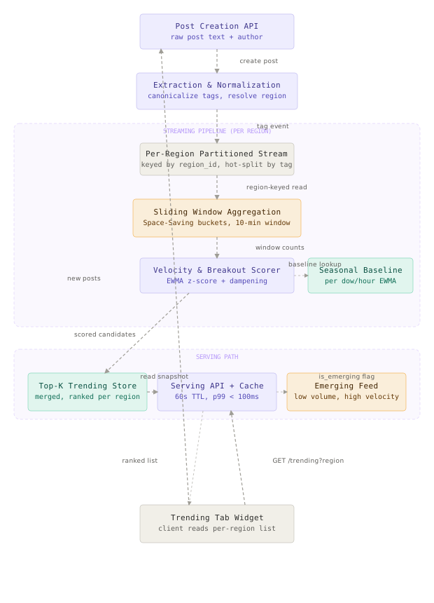
The Ingestion, Extraction and Normalization Layer is the front door for every post: it pulls out raw hashtag substrings, canonicalizes each one so that trivial formatting differences collapse into a single counter, and attaches the resolved region_id. The Per-Region Stream Partitioning Layer routes each normalized hashtag event onto a partition keyed by region, so that a hot region’s volume is physically isolated from every other region’s processing capacity. The Sliding Window Aggregation Engine is the computational core, maintaining a bounded-memory, approximate occurrence count for every hashtag inside each region’s rolling window. The Velocity and Breakout Scoring Engine reads each window’s counts alongside a per-hashtag seasonal baseline and produces a composite score that separates genuine breakouts from predictable recurring spikes. The Top-K Materialization and Serving Layer merges scored candidates into a ranked list per region and answers read requests from a precomputed, cached snapshot rather than from live aggregation state.

A hashtag’s life inside this system looks like this: a post is created, its text is scanned for # tokens, each token is normalized and paired with the post’s resolved region, and that event lands on the region’s stream partition within milliseconds. Once a minute, the aggregation engine closes the current one-minute bucket, folds it into a trailing ten-minute sliding window, and hands the region’s updated counts to the scoring engine. The scoring engine looks up each hashtag’s short-term and seasonal baselines, computes a velocity-aware composite score, applies a dampening multiplier to tags whose spike matches their own predictable historical pattern, and flags tags whose velocity is anomalous relative to their history as emerging even if their raw count is still small. The top-K materializer merges scored candidates across any shards a busy region has been split into, writes the new ranked list to the trending store, and the serving layer’s cache picks it up on the next client read.

Component Deep Dives

The Ingestion, Extraction and Normalization Layer

This component’s job is to turn raw post text into a clean, canonical, region-tagged hashtag event before anything downstream ever counts it.

The mistake a simpler design makes is treating hashtag text as already clean. Real posts produce #WorldCup, #worldcup, #WORLDCUP, and a version with a trailing zero-width joiner pasted in from a copied caption, and if all four are counted as distinct keys, a single trend gets fragmented into four small counters, none of which is large enough to rank, while the tag itself is genuinely huge. Normalization has to run exactly once, at ingestion, so every downstream counter, sketch, and baseline lookup agrees on one canonical key for the same trend.

# Hashtag extraction and canonicalization: runs once at ingestion so
# every downstream stage counts against a single, stable key per trend
import re
import unicodedata

HASHTAG_PATTERN = re.compile(r"#([^\s#.,!?;:()\[\]{}\"']+)", re.UNICODE)
ZERO_WIDTH_CHARS = dict.fromkeys(
    [0x200B, 0x200C, 0x200D, 0xFEFF], None  # ZWSP, ZWNJ, ZWJ, BOM
)
MIN_TAG_LENGTH = 2
MAX_TAG_LENGTH = 64

def extract_hashtags(post_text: str) -> list[str]:
    raw_matches = HASHTAG_PATTERN.findall(post_text)
    seen = set()
    canonical_tags = []
    for raw in raw_matches:
        canonical = canonicalize_hashtag(raw)
        if canonical and canonical not in seen:
            seen.add(canonical)
            canonical_tags.append(canonical)
    return canonical_tags

def canonicalize_hashtag(raw: str) -> str | None:
    stripped = raw.translate(ZERO_WIDTH_CHARS)
    normalized = unicodedata.normalize("NFKC", stripped)
    folded = normalized.casefold()
    folded = folded.strip("_-")
    if not (MIN_TAG_LENGTH <= len(folded) <= MAX_TAG_LENGTH):
        return None
    if not any(ch.isalnum() for ch in folded):
        return None
    return folded

def resolve_region_and_emit(post_id: str, author_id: str, post_text: str,
                             region_id: str, event_ts_ms: int, emit_fn) -> None:
    for canonical_tag in extract_hashtags(post_text):
        emit_fn({
            "post_id": post_id,
            "hashtag": canonical_tag,
            "region_id": region_id,
            "event_ts_ms": event_ts_ms,
        })

Think of this like a librarian who reshelves every incoming book under a single standardized subject heading before it ever reaches the catalog, rather than letting “Sci-Fi”, “SciFi”, and “Science Fiction” each accumulate their own separate, smaller shelf. What breaks without it: #worldcup and #WorldCup compete as two different, smaller entries instead of combining into one large one, and a tag that should clearly be a region’s top trend instead shows up nowhere near the top-K because its true volume is split across lookalike keys.

The Per-Region Stream Partitioning Layer

This component’s job is to route every normalized hashtag event onto a partition keyed by region, so that no region’s processing ever competes with another region’s for the same consumer capacity.

The non-obvious failure of a single shared partitioning scheme is that region sizes are wildly uneven. A handful of large countries generate the bulk of platform volume on an ordinary day, and any one of the roughly 600 regions can spike to several times its own baseline during a national event, a sports final, or breaking news. If regions are partitioned purely by a flat hash of region_id across a fixed partition count, a single busy region can land entirely on one partition and saturate the consumer reading it, while every other region on that same partition falls behind through no fault of its own.

// Partition key assignment for the region-keyed stream: ordinary
// regions get a fixed number of partitions, but a region flagged as
// hot is sub-partitioned by a hash of the hashtag itself, spreading
// its load across multiple partitions instead of one
package streaming

import (
	"hash/fnv"
)

const basePartitionCount = 64
const hotRegionSubPartitions = 8

type HashtagEvent struct {
	RegionID string
	Hashtag  string
}

func partitionKey(event HashtagEvent, hotRegions map[string]bool) uint32 {
	h := fnv.New32a()
	if hotRegions[event.RegionID] {
		h.Write([]byte(event.RegionID))
		h.Write([]byte(event.Hashtag))
		subPartition := h.Sum32() % hotRegionSubPartitions
		return regionBasePartition(event.RegionID) + subPartition
	}
	h.Write([]byte(event.RegionID))
	return h.Sum32() % basePartitionCount
}

func regionBasePartition(regionID string) uint32 {
	h := fnv.New32a()
	h.Write([]byte(regionID))
	return (h.Sum32() % basePartitionCount) * hotRegionSubPartitions
}

# Kafka topic definition for the region-partitioned hashtag stream
name: hashtag-events-by-region
partitions: 512
replication_factor: 3
retention_ms: 86400000
compression_type: lz4
config:
  min.insync.replicas: 2
  max.message.bytes: 4096

This is the same trick a highway system uses when a stadium empties out after a game: ordinary traffic uses the regular lanes, but the moment volume spikes near one exit, temporary contraflow lanes open specifically for that exit so the surge does not back up traffic for every other exit on the same highway. What breaks without hot-region sub-partitioning: a single viral event in one country can push consumer lag for that country’s partition into the minutes, and because the aggregation engine’s one-minute cadence depends on timely reads, that region’s trending list goes stale exactly when its readers care about freshness the most.

The Sliding Window Aggregation Engine

This component’s job is to maintain an approximate, bounded-memory occurrence count for every hashtag inside each region’s rolling window, without that memory budget growing as new hashtags appear.

The instinct to keep an exact count per hashtag in a hash map is reasonable until you account for the tail. On a single busy day, tens of millions of distinct hashtags appear across the platform, the overwhelming majority used only once or twice, and an exact counter never forgets a key once it has seen it. A process holding one hash map per region for an unbounded key space eventually runs out of memory, and it does so unpredictably, since the growth rate depends on how creative that day’s posts happen to be, not on anything the operator controls. The fix is a heavy-hitters sketch with a fixed counter budget: the Space-Saving algorithm, which guarantees that any hashtag whose true count is large enough to matter is tracked with a bounded overestimate, while genuinely rare tags are evicted without ever growing the structure past its configured size.

# Space-Saving heavy hitters: bounded-memory approximate counting
# that guarantees any sufficiently frequent hashtag is tracked, with
# a provable upper bound on the overestimation error
class SpaceSavingCounter:
    def __init__(self, capacity: int = 2000):
        self.capacity = capacity
        self.counts: dict[str, int] = {}
        self.error: dict[str, int] = {}

    def add(self, key: str, increment: int = 1) -> None:
        if key in self.counts:
            self.counts[key] += increment
            return
        if len(self.counts) < self.capacity:
            self.counts[key] = increment
            self.error[key] = 0
            return
        # Evict the current minimum, its slot's error bound absorbs
        # the incoming key's uncertainty going forward
        min_key = min(self.counts, key=self.counts.get)
        min_count = self.counts.pop(min_key)
        self.error.pop(min_key)
        self.counts[key] = min_count + increment
        self.error[key] = min_count

    def top_k(self, k: int) -> list[tuple[str, int, int]]:
        ranked = sorted(self.counts.items(), key=lambda kv: kv[1], reverse=True)
        return [(key, count, self.error[key]) for key, count in ranked[:k]]

class RegionWindow:
    """Ring buffer of one-minute Space-Saving buckets rolled into a
    trailing ten-minute sliding window per region."""
    def __init__(self, bucket_count: int = 10, bucket_capacity: int = 2000):
        self.bucket_count = bucket_count
        self.bucket_capacity = bucket_capacity
        self.buckets: list[SpaceSavingCounter] = [
            SpaceSavingCounter(bucket_capacity) for _ in range(bucket_count)
        ]
        self.write_index = 0

    def record(self, hashtag: str) -> None:
        self.buckets[self.write_index].add(hashtag)

    def roll_bucket(self) -> None:
        # Advance to the next bucket, overwriting the oldest one and
        # evicting it from the trailing ten-minute window
        self.write_index = (self.write_index + 1) % self.bucket_count
        self.buckets[self.write_index] = SpaceSavingCounter(self.bucket_capacity)

    def windowed_counts(self) -> dict[str, int]:
        merged: dict[str, int] = {}
        for bucket in self.buckets:
            for key, count in bucket.counts.items():
                merged[key] = merged.get(key, 0) + count
        return merged

Think of each one-minute bucket like a single tray on a sushi conveyor belt: a fixed number of trays circle past, a new tray is added at one end while the oldest tray is removed at the other, and at any moment the current view is just whatever trays happen to be on the belt right now, no matter how many have passed by over the course of the day. What breaks without bucketed rolling: computing a ten-minute window by re-scanning every raw event that arrived in the last ten minutes means storage and compute both grow with raw event volume, whereas ten fixed-capacity buckets keep the memory footprint constant regardless of how many events actually occurred.

The Velocity and Breakout Scoring Engine

This component’s job is to turn a region’s windowed hashtag counts into a ranked score that rewards genuine acceleration, not just size, and separates predictable recurring spikes from real breakouts.

The non-obvious part is that “high count” and “high velocity” are different signals, and conflating them produces a chart dominated by tags that are simply always large, sports team names, generic greetings, popular shows, none of which is what a reader opens a trending tab to discover. Velocity has to be measured against each hashtag’s own recent behavior, using a fast-moving short-horizon average compared against a slower long-horizon average, so a tag accelerating away from its own normal shows up even while its absolute count is still modest.

# EWMA-based velocity and breakout scoring: compares a fast-moving
# baseline against a slow-moving one so acceleration is detected
# relative to each hashtag's own recent history, not a flat threshold
import math

SHORT_ALPHA = 0.5     # short EWMA reacts within ~2 windows
LONG_ALPHA = 0.05      # long EWMA reacts over ~20 windows
MIN_VOLUME_FOR_RANKING = 15
EMERGING_ZSCORE_THRESHOLD = 3.0
EMERGING_MAX_VOLUME = 200

class HashtagBaseline:
    __slots__ = ("short_ewma", "long_ewma", "long_variance")
    def __init__(self, short_ewma: float = 0.0, long_ewma: float = 0.0,
                 long_variance: float = 1.0):
        self.short_ewma = short_ewma
        self.long_ewma = long_ewma
        self.long_variance = long_variance

def update_baseline(baseline: HashtagBaseline, current_count: int) -> HashtagBaseline:
    deviation = current_count - baseline.long_ewma
    new_long_variance = (
        (1 - LONG_ALPHA) * baseline.long_variance
        + LONG_ALPHA * (deviation ** 2)
    )
    return HashtagBaseline(
        short_ewma=(1 - SHORT_ALPHA) * baseline.short_ewma + SHORT_ALPHA * current_count,
        long_ewma=(1 - LONG_ALPHA) * baseline.long_ewma + LONG_ALPHA * current_count,
        long_variance=max(new_long_variance, 1.0),
    )

def velocity_zscore(baseline: HashtagBaseline) -> float:
    std_dev = math.sqrt(baseline.long_variance)
    return (baseline.short_ewma - baseline.long_ewma) / std_dev

def composite_score(current_count: int, baseline: HashtagBaseline,
                     dampening_multiplier: float,
                     volume_weight: float = 0.6, velocity_weight: float = 0.4) -> dict:
    if current_count < MIN_VOLUME_FOR_RANKING:
        return {"score": 0.0, "is_emerging": False}

    zscore = velocity_zscore(baseline)
    volume_norm = min(math.log1p(current_count) / math.log1p(50_000), 1.0)
    velocity_norm = min(max(zscore, 0.0) / 8.0, 1.0)

    raw_score = (volume_weight * volume_norm + velocity_weight * velocity_norm)
    score = raw_score * dampening_multiplier

    is_emerging = (
        zscore >= EMERGING_ZSCORE_THRESHOLD
        and current_count <= EMERGING_MAX_VOLUME
    )
    return {"score": score, "zscore": zscore, "is_emerging": is_emerging}

Think of this like comparing a car’s current speed not to a fixed speed limit but to its own recent average speed on the same stretch of road at the same time of day. A car doing 60 on a highway is unremarkable, but a car that has averaged 20 on that stretch for weeks and just jumped to 60 in the last few minutes is the one worth flagging, and that is exactly the deviation the short-versus-long EWMA comparison detects. What breaks without a dual-horizon comparison: a single flat volume threshold either misses genuinely small but fast-accelerating breakouts entirely, since they never reach the threshold in the window that matters, or it floods the list with tags that are simply always big.

The Top-K Materialization and Serving Layer

This component’s job is to merge scored candidates, including any produced by a hot region’s multiple sub-partitions, into one ranked list per region and serve it with low, predictable latency.

The mistake a simpler design makes is assuming top-K selection can happen on a single node holding the whole region’s data. Once a region is hot enough to need the sub-partitioning described earlier, its hashtag counts are split across several shards, and no single shard has the true global count for any one hashtag. The Space-Saving structure’s mergeability is what rescues this: two Space-Saving summaries over disjoint slices of the same key space can be combined into a summary of the union, with the same provable error bound, which is exactly what a naive exact top-K cannot do without re-scanning everything.

# Merging shard-local Space-Saving summaries into one region-level
# top-K, exploiting the algorithm's mergeability so a hot region's
# sub-partitions never need to funnel through a single bottleneck node
def merge_shard_summaries(shard_summaries: list[SpaceSavingCounter],
                           merged_capacity: int = 2000) -> SpaceSavingCounter:
    merged = SpaceSavingCounter(merged_capacity)
    all_keys: set[str] = set()
    for summary in shard_summaries:
        all_keys.update(summary.counts.keys())

    for key in all_keys:
        total = 0
        max_error = 0
        for summary in shard_summaries:
            if key in summary.counts:
                total += summary.counts[key]
            else:
                # Key absent from this shard: its true count there is
                # unknown but bounded by that shard's own error margin
                total += 0
                max_error = max(max_error, summary_min_count(summary))
        merged.counts[key] = total
        merged.error[key] = max_error

    if len(merged.counts) > merged_capacity:
        trimmed = sorted(merged.counts.items(), key=lambda kv: kv[1], reverse=True)
        keep = dict(trimmed[:merged_capacity])
        merged.counts = keep
        merged.error = {k: merged.error[k] for k in keep}
    return merged

def summary_min_count(summary: SpaceSavingCounter) -> int:
    return min(summary.counts.values()) if summary.counts else 0

def materialize_top_k(region_id: str, scored_candidates: list[dict], k: int = 50) -> list[dict]:
    ranked = sorted(scored_candidates, key=lambda c: c["score"], reverse=True)[:k]
    return [
        {"region_id": region_id, "rank": i + 1, **candidate}
        for i, candidate in enumerate(ranked)
    ]

This is the same principle a chain of regional warehouses uses when producing a national top-sellers report: each warehouse keeps its own accurate local tally, and headquarters combines those tallies into a national ranking without ever needing one warehouse to hold every other warehouse’s inventory records. What breaks without mergeability: a hot region split for load reasons would need a second, separate coordination step just to answer “what’s actually trending here,” reintroducing exactly the single-node bottleneck that sub-partitioning was meant to eliminate.

Data Model

The data model spans four core entities: normalized hashtag events, windowed counts, seasonal baselines, and trending snapshots.

-- Normalized hashtag events: the durable log the aggregation engine
-- consumes; retained briefly for replay, not as a query surface
CREATE TABLE hashtag_events (
    event_id       BIGINT      NOT NULL,
    post_id        BIGINT      NOT NULL,
    region_id      TEXT        NOT NULL,
    hashtag        TEXT        NOT NULL,
    event_ts       TIMESTAMPTZ NOT NULL,
    PRIMARY KEY (region_id, event_ts, event_id)
);

-- Windowed counts: the materialized output of each region's rolling
-- ten-minute window, written once per one-minute tick
CREATE TABLE hashtag_window_counts (
    region_id      TEXT        NOT NULL,
    hashtag        TEXT        NOT NULL,
    window_end     TIMESTAMPTZ NOT NULL,
    window_count   BIGINT      NOT NULL CHECK (window_count >= 0),
    error_bound    BIGINT      NOT NULL DEFAULT 0,
    PRIMARY KEY (region_id, hashtag, window_end)
);

CREATE INDEX ON hashtag_window_counts (region_id, window_end);

-- Seasonal baselines: per-hashtag, per-region expected volume and
-- velocity keyed by day-of-week and hour-of-day, used for dampening
CREATE TABLE hashtag_seasonal_baseline (
    region_id       TEXT             NOT NULL,
    hashtag         TEXT             NOT NULL,
    day_of_week     SMALLINT         NOT NULL CHECK (day_of_week BETWEEN 0 AND 6),
    hour_of_day     SMALLINT         NOT NULL CHECK (hour_of_day BETWEEN 0 AND 23),
    ewma_count      DOUBLE PRECISION NOT NULL DEFAULT 0,
    ewma_variance   DOUBLE PRECISION NOT NULL DEFAULT 1,
    updated_at      TIMESTAMPTZ      NOT NULL DEFAULT NOW(),
    PRIMARY KEY (region_id, hashtag, day_of_week, hour_of_day)
);

-- Trending snapshots: the top-K materialized result the serving
-- layer actually reads, one row per ranked hashtag per tick
CREATE TABLE trending_snapshot (
    region_id         TEXT             NOT NULL,
    rank               SMALLINT         NOT NULL CHECK (rank BETWEEN 1 AND 50),
    hashtag            TEXT             NOT NULL,
    window_count       BIGINT           NOT NULL,
    velocity_zscore    DOUBLE PRECISION NOT NULL,
    composite_score    DOUBLE PRECISION NOT NULL,
    is_emerging        BOOLEAN          NOT NULL DEFAULT FALSE,
    computed_at        TIMESTAMPTZ      NOT NULL,
    PRIMARY KEY (region_id, computed_at, rank)
);

CREATE INDEX ON trending_snapshot (region_id, computed_at DESC);

hashtag_window_counts and hashtag_seasonal_baseline are both sharded by region_id, matching the partitioning key used everywhere upstream, so a shard never needs another shard’s data to compute one region’s ranking. trending_snapshot is also sharded by region_id, and the serving layer’s read is always region_id plus the most recent computed_at, a single-partition lookup with no cross-shard fan-out.

A hashtag event’s life starts the moment a post is created: it lands in hashtag_events as a durable, replayable log, and within the same second it is folded into the current one-minute Space-Saving bucket for its region. Once a minute, the bucket rolls, the trailing ten-minute window is recomputed and written to hashtag_window_counts, and the scoring engine reads that row alongside the matching hashtag_seasonal_baseline row for the current day-of-week and hour-of-day. The scoring engine writes an updated ewma_count and ewma_variance back to the baseline table, closing the feedback loop that keeps future dampening accurate, and writes the ranked result into trending_snapshot. From there the serving layer’s cache picks up the newest computed_at row per region on the next client read.

Key Algorithms and Protocols

Hashtag Normalization and Canonicalization

Covered in the Ingestion, Extraction and Normalization Layer section above, this algorithm runs in O(length of post text) per post and is idempotent: applying it twice to an already-canonical tag returns the same tag.

Space-Saving Heavy Hitters for Bounded-Memory Sliding Windows

Covered in the Sliding Window Aggregation Engine section above, each add runs in O(1) amortized time using a hash map plus a lazily maintained minimum, and the structure never exceeds its configured capacity, regardless of how many distinct hashtags it has observed.

Seasonal Dampening for Recurring Tags

The dampening step compares a hashtag’s current velocity not against a single global normal, but against that exact hashtag’s own historical pattern at this day-of-week and hour-of-day. A tag whose current spike closely matches its usual Monday-morning shape gets its score suppressed; a tag spiking well beyond its own historical pattern for this slot does not.

# Dampening multiplier: suppresses a hashtag's score in proportion to
# how closely today's spike matches its own historical pattern for
# this exact day-of-week and hour-of-day slot
DAMPENING_FLOOR = 0.15  # a perfectly matched recurring spike is never zeroed out entirely
MATCH_TOLERANCE = 1.5   # in units of historical standard deviation

def dampening_multiplier(current_count: int, seasonal_ewma: float,
                          seasonal_std_dev: float) -> float:
    if seasonal_ewma <= 0:
        return 1.0  # no seasonal history yet, apply no dampening

    deviation_from_seasonal_norm = abs(current_count - seasonal_ewma) / max(seasonal_std_dev, 1.0)

    if deviation_from_seasonal_norm <= MATCH_TOLERANCE:
        # Spike matches this slot's own history closely: heavily dampen
        return DAMPENING_FLOOR
    # Spike exceeds this slot's own history: dampening fades out as the
    # excess grows, approaching 1.0 for a genuinely unprecedented spike
    excess = deviation_from_seasonal_norm - MATCH_TOLERANCE
    return min(DAMPENING_FLOOR + (excess / 6.0), 1.0)

Mergeable Top-K Across Shards

Covered in the Top-K Materialization and Serving Layer section above, merging n shard summaries each of capacity m runs in O(n * m) time and produces a result with the same provable error bound as a single Space-Saving structure over the full combined stream.

Scaling and Performance

The Sliding Window Aggregation Engine and the stream partitioning layer feeding it carry the tightest resource budget in this system, since every hashtag instance across roughly 600 regions has to be folded into a bucket within the same one-minute tick that produces the next trending refresh.

Ordinary regions run comfortably on a single partition and a single aggregation worker. A region crosses into hot status when its sustained event rate exceeds a configured threshold relative to its own baseline, at which point its traffic is re-keyed across hotRegionSubPartitions using the hashtag itself as the secondary hash, spreading load evenly regardless of which individual tags happen to be driving the spike. Demoting a region back to a single partition once its volume subsides is the mirror operation, and both transitions are safe specifically because the Space-Saving summaries involved are mergeable in either direction.

Capacity Estimation:

Given:
  - ~500 million posts/day platform-wide
  - ~32% of posts contain at least one hashtag -> ~160M tagged posts/day
  - ~1.7 hashtags per tagged post -> ~272M hashtag instances/day
  - ~600 tracked regions
  - Hot region burst: up to 8x a region's own baseline rate
  - Sliding window: 10 buckets of 1 minute each, refreshed every 60s
  - Top-K per region: top 50, plus a separate emerging feed

Average ingestion rate:
  272,000,000 / 86,400 seconds = ~3,150 hashtag instances/sec average

Peak ingestion rate:
  platform-wide peak ~3x average = ~9,500/sec, with an individual hot
  region additionally spiking up to 8x its own local baseline

Raw event bandwidth:
  ~272M events/day * ~120 bytes/event (post_id, hashtag, region_id,
  timestamp) = ~32.6 GB/day raw, ~98 GB/day at 3x Kafka replication

Space-Saving memory footprint:
  600 regions * 2,000 counters/region * ~40 bytes/counter
  (hashtag string + count + error bound) = ~48 MB total resident
  across all region summaries, trivially held in memory with room
  for replication across multiple aggregation nodes for failover

Trending snapshot writes:
  600 regions * 50 ranked rows * 1 write/minute * 1,440 minutes/day
  = ~43.2M rows/day, at ~80 bytes/row = ~3.5 GB/day

Serving read volume:
  ~45,000 trending-list reads/sec at peak, served entirely from a
  cache in front of `trending_snapshot`, targeting p99 under 100ms

The trending snapshot is read-heavy and write-once-per-minute, which makes it an easy target for aggressive caching: a short-TTL, sixty-second cache in front of trending_snapshot, invalidated naturally by the next tick’s write, absorbs nearly all read traffic without the serving layer ever touching the underlying store on a cache hit. The dominant bottleneck is not aggregate read volume, which is modest, it is keeping the aggregation engine’s per-tick work bounded across a region population whose individual volumes can vary by orders of magnitude and shift dramatically within minutes.

Failure Modes and Recovery

Failure	Detection	Impact	Recovery
A hot region’s consumer lag grows during an unanticipated spike before hot-region sub-partitioning kicks in	Consumer lag metric per partition crossing a threshold	That region’s trending list falls behind the 60-90 second freshness target	Auto-promotion to hot-region sub-partitioning triggers on lag, not just raw rate, backfilling from the retained event log once caught up
A burst of coordinated bot posting artificially inflates one hashtag’s count in a single region	Anomaly detector flags an unusually narrow distribution of post_id author accounts behind one hashtag’s spike	A spam-driven tag displaces a genuine trend in the top-K	The scoring engine applies an author-diversity discount, a spike concentrated among few distinct authors is down-weighted before ranking, independent of the upstream spam filter
The seasonal baseline update job falls behind or fails for a region	Baseline write staleness alert per region	Dampening uses a stale baseline, recurring tags may not be suppressed correctly that day	Scoring falls back to the last successfully written baseline snapshot rather than blocking; a stale-but-present baseline degrades gracefully instead of disabling dampening entirely
A region is geo-misclassified for a batch of posts, for example VPN traffic resolving to the wrong country	Spike in low-confidence region resolutions from the upstream geo-resolution signal	Hashtags leak into a region’s trending list that do not actually reflect that region’s activity	Posts with low-confidence region resolution route to a global-unclassified bucket instead of a specific region, excluded from any single region’s ranking
A Space-Saving summary for a region grows corrupted or is lost on aggregation node failure	Heartbeat and checksum mismatch from the aggregation worker	That region produces no valid trending update for the current tick	The event log retains enough history to replay the current window from hashtag_events, rebuilding the summary on a fresh worker within one tick’s worth of catch-up
The trending snapshot write for a region completes only partially mid-tick	Row-count reconciliation between expected top-K size and rows actually written	Readers could see a truncated or inconsistent ranked list	The materializer writes a full tick’s rows under a single computed_at value and the serving layer only ever reads the newest fully-committed computed_at, so a partial write is simply never exposed to readers

Comparison of Approaches

Approach	Latency	Complexity	Failure mode	Best fit
Streaming approximate counting with velocity and seasonal dampening, region-sharded (this design)	Read path under 100ms; freshness within 60-90 seconds	High, requires a heavy-hitters sketch, dual-horizon baselines, and hot-region sub-partitioning	A misconfigured dampening threshold can over-suppress a genuine recurring-shaped surprise	Platforms with hundreds of regions and hashtag cardinality too large for exact counting to stay memory-bounded
Exact per-hashtag counting in a relational store with a GROUP BY per window	Degrades as cardinality grows; can exceed the freshness target under load	Low to build initially	Table and index size grow without bound as new hashtags appear, eventually forcing manual pruning or crashing under memory pressure	Small platforms or a single region with a hashtag vocabulary that stays in the low millions
Pure raw-volume top-K, no velocity or dampening	Fast to compute, same infrastructure as this design minus the scoring stage	Low	Recurring ritual tags permanently occupy trending slots; breakouts are only visible once they are already large	A minimal viable version where launch speed matters more than trend quality
Hourly or daily batch recomputation instead of a streaming pipeline	Freshness measured in hours, far outside the 60-90 second target	Medium, simpler than streaming infrastructure	An event that spikes and fades entirely within an hour can be missed by the batch window altogether	Lower-traffic platforms where near-real-time trending is not a product requirement
Global trending computed once, then filtered per region after the fact	Fast for a single global computation	Low	Genuinely large regional trends that are not globally significant never surface, since they lose to global volume before regional filtering ever happens	Platforms with one dominant, culturally homogeneous market and no real need for regional differentiation

We would pick the streaming, region-sharded design with velocity and seasonal dampening for a platform at this scale, because it is the only approach here that keeps freshness inside a minute while remaining memory-bounded against an effectively unlimited hashtag vocabulary. Exact counting and batch recomputation both reintroduce a resource or freshness ceiling that a growing platform eventually hits, and post-hoc global-to-regional filtering throws away the entire reason regional trending exists in the first place, surfacing what is genuinely significant locally, not just locally visible.

Key Takeaways

• Velocity, not volume, is the leading indicator of a genuine breakout. A hashtag’s raw count tells you what already happened; comparing its short-horizon average against its own long-horizon baseline tells you what is happening right now.
• Region has to be the sharding key from ingestion through serving, not a filter bolted onto a global result. That is what lets one region’s 8x traffic spike stay fully isolated from every other region’s freshness.
• Bounded-memory approximate counting is what makes an unbounded hashtag vocabulary tractable. Space-Saving’s provable error bound means the system trades a small, quantifiable amount of precision for a memory footprint that never grows with cardinality.
• Dampening needs each hashtag’s own seasonal baseline, not one global threshold. A tag’s Monday-morning spike looks identical in raw count to a genuine breakout; only comparing it against its own history for that exact slot tells the two apart.
• Mergeability is what makes hot-region sub-partitioning safe. Splitting a busy region’s load across shards costs nothing in ranking correctness precisely because Space-Saving summaries can be combined with the same error guarantees as a single unsplit structure.
• Normalization has to happen exactly once, at ingestion. Every downstream sketch, baseline, and score depends on every occurrence of the same real-world trend arriving under one canonical key.
• Freshness at a one-minute cadence is a deliberate cost tradeoff, not a hard technical limit. The marginal value of a tighter cadence is small relative to its compute cost, so the budget goes toward a wider, more reliable sliding window instead.
• Serving and aggregation are different problems solved by different systems. The aggregation engine optimizes for bounded per-tick compute across hundreds of regions; the serving layer optimizes for p99 latency on one cached, precomputed row.

The counter-intuitive lesson is that the part of this system that sounds hardest, counting hashtag occurrences across an unbounded vocabulary at platform scale, is the well-understood part with a textbook algorithmic answer. The genuinely hard part is defining what “trending” should even mean for a single hashtag over time, distinguishing a spike that is merely that tag’s ordinary Monday from one that is actually new, which is why the seasonal dampening layer, not the counting layer, is where most of this design’s real judgment calls live.

Frequently Asked Questions

Q: Why not just rank hashtags by raw count in the current window and skip velocity scoring entirely?

A: Raw count rewards tags that are simply always large, generic greetings, popular ongoing shows, well-known team names, crowding out the surprising, newly emerging stories a trending feature exists to surface. Velocity, comparing a fast-moving short-term average against a slower long-term baseline, is what lets a tag with modest absolute volume but sharp acceleration outrank a tag that is merely consistently big.

Q: Why use an approximate counting structure like Space-Saving instead of exact per-hashtag counters?

A: Tens of millions of distinct hashtags appear across a single day, the overwhelming majority used once or twice, and an exact counter never forgets a key once it has seen it, so its memory footprint grows without bound as the vocabulary grows. Space-Saving caps memory at a fixed counter budget per region and guarantees that any hashtag frequent enough to matter is tracked with a provable, bounded overestimate, trading a small amount of precision on the irrelevant long tail for a memory footprint that never grows.

Q: How do you stop a single massive global event from swamping every region’s trending list at once?

A: It cannot, by construction, because every stage of the pipeline, partitioning, aggregation, and scoring, operates per region. A globally significant event will independently earn a top rank in each region where it is genuinely driving velocity, but a region where that event has little local traction simply will not surface it, since that region’s baselines and rankings are computed entirely from its own traffic.

Q: How is a post’s region actually determined, and what happens when the signal is unreliable, like VPN traffic?

A: Region resolution is an upstream responsibility, generally a geo-IP lookup blended with a user’s declared locale when available, and this system consumes a region_id plus a confidence signal rather than computing resolution itself. Posts with low-confidence resolution are routed to a separate global-unclassified bucket rather than guessed into a specific region, since a wrongly attributed post can distort a smaller region’s counts far more than a correctly excluded one costs in coverage.

Q: Why maintain a per-hashtag seasonal baseline instead of one global definition of “normal” volume?

A: A single global normal cannot distinguish a small hashtag’s ordinary daily rhythm from a large hashtag’s ordinary daily rhythm, and both look like deviations from a flat threshold at different points in the day. Keying the baseline by hashtag, region, day-of-week, and hour lets each tag be judged against its own history, which is the only way to correctly dampen a genuinely recurring tag without also dampening a different tag’s first-ever appearance at that same hour.

Q: How does the system avoid promoting a hashtag that is trending only because of coordinated bot or spam activity?

A: Upstream spam and bot filtering removes the bulk of obviously fraudulent traffic before it reaches this pipeline, but the scoring engine adds its own defense: a spike concentrated among an unusually narrow set of distinct authors is discounted before ranking, independent of whatever the upstream filter caught or missed, since organic breakouts are almost always driven by a broad, diverse set of authors rather than a small coordinated cluster.

Interview Questions

Q: Design the sliding window structure that lets you compute both a one-minute and a ten-minute view of hashtag volume per region without storing every raw event indefinitely.

Expected depth: Cover a ring buffer of fixed-size one-minute buckets, each backed by a bounded heavy-hitters sketch, rolling the oldest bucket out as a new one is written, and merging the current set of buckets on demand to produce the trailing window, versus the alternative of re-scanning raw events, and why the fixed-bucket approach keeps both memory and per-tick compute constant.

Q: How would you detect an emerging breakout hashtag that has only 40 mentions in a region with millions of daily active users?

Expected depth: Discuss comparing a short-horizon EWMA against a long-horizon EWMA to compute a z-score independent of absolute volume, an explicit low-volume ceiling that keeps the emerging feed distinct from the main top-K, and the tradeoff of a low minimum-volume floor catching more genuine early breakouts at the cost of more noise from statistically small samples.

Q: Design the dampening mechanism for a hashtag like a Monday-motivation tag that spikes on a predictable weekly schedule.

Expected depth: Cover keying a seasonal baseline by hashtag, region, day-of-week, and hour, comparing today’s count against that specific slot’s historical EWMA and variance rather than a flat threshold, a dampening multiplier that fades toward full weight as the deviation from the seasonal norm grows, and why the baseline needs to be updated continuously rather than fixed once, so a tag whose pattern changes over time is not permanently mis-dampened.

Q: A single country experiences 8x normal post volume during a national election. Walk through what happens to that region’s aggregation pipeline and how you prevent it from starving other regions.

Expected depth: Discuss consumer lag as the trigger for promoting a region to hot-region status, sub-partitioning that region’s stream by a secondary hash of the hashtag itself, running Space-Saving summaries independently per sub-partition, and merging them back into one region-level top-K using the structure’s mergeability, all without any other region’s partitions or consumers being affected.

Q: How would you extend this system to detect a hashtag trending across many regions simultaneously, a genuinely global trend, versus one confined to a single region?

Expected depth: Cover an additional aggregation tier that reads each region’s already-computed scores rather than raw events, counting how many regions independently rank a given hashtag above some threshold within the same tick, the distinction between a globally coordinated event and many regions independently discovering the same tag for unrelated local reasons, and why this tier should consume per-region output instead of re-running velocity scoring against a flattened global stream.