Build an Imbalanced Fraud Classifier with SMOTE and Cost-Sensitive Learning
classical-ml fraud-detection model-evaluation feature-engineering View full code for this problem
ML Problem & Solution
Fraud Detection Under Extreme Class Imbalance
0.17% positives, a 40ms budget, and a metric that rewards a model for doing nothing at all
A payments platform processes 2.1 million card-not-present transactions a month, and roughly 3,600 of them are fraudulent. That is a base rate of 0.17%. When fraud gets through, the issuing bank claws the money back as a chargeback and the platform eats the loss: 187 dollars on average, plus a 15 dollar network fee and an operational cost that nobody wants to itemize. When the platform blocks a legitimate transaction instead, the cost is smaller but not zero: an estimated 4.30 dollars in lost margin, support contact, and the measurable probability that the customer does not come back.
The imbalance is the entire problem, and it poisons the obvious approach in two separate ways. First, it makes the default metric useless. A model that predicts “not fraud” for every single transaction scores 99.83% accuracy, beats most honest first attempts, and prevents zero dollars of loss. Second, it makes the default loss function useless. Log loss averaged over 2.1 million rows is dominated by the 2,096,400 easy negatives, so gradient descent spends nearly all its capacity getting confident about transactions nobody was worried about. The 3,600 rows that carry all the business value contribute about 0.17% of the gradient signal.
There is a third problem that only shows up after you ship. Fraud labels arrive late. A chargeback is filed 45 to 120 days after the transaction, which means the most recent three months of data have artificially low fraud rates simply because the chargebacks have not landed yet. Train on a window that includes immature labels and the model learns that recent transactions are safe, which is the opposite of true. And fraud is adversarial: the patterns that predicted fraud last quarter are the ones that got blocked, so the fraudsters moved. The data-generating process actively fights the model, unlike house prices or churn.
Think of it as airport security screening where 1 in 600 passengers is carrying something, you have twelve inspectors, and an inspection costs the airline a small amount of goodwill while a miss costs it an aircraft. Nobody in that building cares about the fraction of passengers correctly waved through. They care about how much contraband those twelve inspectors catch per shift, and letting the queue grow past the terminal doors is not an option.
Given a card-not-present transaction with its merchant, card, device, and historical-velocity features available at authorization time, output a fraud probability, optimizing expected net loss in dollars, under a 40ms p99 scoring budget and a hard ceiling of 1,800 manual reviews per day.
Framing the Problem
This is binary classification with a severely skewed prior and asymmetric, known misclassification costs. That second clause matters more than the first. Class imbalance is a nuisance; asymmetric costs are the actual objective. Once you write the cost matrix down, most of the standard imbalance advice reorganizes itself around it.
The target is is_fraud, defined as: the transaction received a chargeback with reason code in the fraud family (10.4, 10.5, 4837, 4863) within 120 days of authorization, OR it was confirmed fraudulent by the cardholder during a support contact. Friendly fraud, where the cardholder genuinely bought the thing and then disputed it, uses a different reason code family and is deliberately excluded. Conflating the two teaches the model to predict buyer’s remorse, which no amount of device fingerprinting will ever capture.
Label maturity is the definition detail that breaks pipelines. A transaction is only labelable once 120 days have passed. We therefore hold out the most recent 120 days entirely and train on the window before it:
# Label maturity gate: only transactions old enough to have final chargeback status.
import pandas as pd

MATURITY_DAYS = 120
as_of = pd.Timestamp("2026-09-01")

txns = pd.read_parquet("data/transactions.parquet")
mature = txns[txns["auth_ts"] <= as_of - pd.Timedelta(days=MATURITY_DAYS)].copy()
immature = txns[txns["auth_ts"] > as_of - pd.Timedelta(days=MATURITY_DAYS)]

print(f"mature rows      : {len(mature):,}  fraud rate {mature['is_fraud'].mean():.4%}")
print(f"immature (unused): {len(immature):,} fraud rate {immature['is_fraud'].mean():.4%}")
On our data that prints a mature fraud rate of 0.171% and an immature rate of 0.062%. The immature window looks two and a half times safer purely because the chargebacks have not arrived. Every row of it is poison for training and gold for monitoring.
Constraints
- Latency: 40ms p99 for the full scoring path, including feature retrieval. The model itself gets about 12ms.
- Review capacity: 1,800 human reviews per day, against roughly 70,000 daily transactions. So at most 2.6% of traffic can be sent to a human.
- Decline rate guardrail: the block rate on legitimate traffic must stay under 0.35%. Above that, merchant complaints and authorization-rate regressions outweigh fraud savings.
- Explainability: every decline must carry a reason code for the merchant dashboard and for regulatory response. Global feature importance is not enough; per-decision attribution is required.
- Online scoring: features must be computable from a feature store at authorization time. Anything requiring a batch join that lands tomorrow is unusable.
The optimized metric is PR-AUC (average precision) for model selection, and net fraud cost per 1,000 transactions for the shipping decision. Accuracy is banned outright: the all-negative model scores 99.83% on it. ROC-AUC is nearly as bad here, because with 99.83% negatives, moving from 20,000 to 200,000 false positives barely moves the false positive rate but destroys precision.
Guardrail metrics we must not regress: legitimate-traffic decline rate (under 0.35%), review queue volume (under 1,800 per day), and calibration error on the score used for the expected-cost threshold. Out of scope for this post: graph and network features over shared devices and cards, which are the single largest additional lift available and deserve their own treatment; account-takeover detection, which is a different label; and real-time model updating.
Class imbalance is not one problem, it is three: a metric problem, a gradient problem, and a decision-threshold problem. Resampling only touches the second one, which is why teams who reach for SMOTE first and stop there usually end up disappointed.
Data and Features
The training window is 14 months of mature transactions: 24.8 million rows, 41 raw columns, with 42,400 positives. Sources are the authorization log (transaction attributes), the card and customer dimension tables, a device fingerprint service, and the chargeback ledger that supplies labels.
Fraud features fall into four families, and the second one carries most of the signal.
| Family | Examples | Notes |
|---|---|---|
| Transaction attributes | amount, currency, mcc, is_recurring, entry_mode |
Cheap, weak individually. amount is bimodal for fraud: card testing at under 2 dollars, cash-out at over 400. |
| Velocity and aggregates | transactions per card in last 1h/24h/7d, distinct merchants per device in 24h, amount z-score versus the card’s 90-day mean | Highest signal. Must be computed as of authorization time. |
| Entity reputation | historical fraud rate of the merchant, BIN, device, shipping postcode | Requires smoothing, leaks badly if done naively. |
| Mismatch and geometry | billing-versus-shipping country match, IP-versus-BIN country distance, hour-of-day in cardholder local time | Interaction-shaped; tree models pick these up for free. |
The leakage risk that will get you
Entity reputation features are a trap that catches experienced people. The natural way to build “merchant fraud rate” is a groupby('merchant_id')['is_fraud'].mean() over the training set. That value includes the current row’s own label. For a merchant with 30 transactions and 2 frauds, the feature for one of those fraud rows encodes “this row is fraud” at a strength of 1/30, and gradient boosting will find it. Offline PR-AUC jumps to 0.81, production performance is unchanged, and you spend three weeks wondering why.
The fix is a time-shifted, out-of-fold expanding aggregate with smoothing toward the global prior:
# Leak-free entity reputation: expanding mean strictly before the current row, smoothed.
import numpy as np
import pandas as pd

def expanding_fraud_rate(df: pd.DataFrame, key: str, prior_weight: float = 200.0) -> pd.Series:
    """Fraud rate of `key` using only rows strictly earlier in time, smoothed to the global prior."""
    d = df.sort_values("auth_ts")
    grp = d.groupby(key, sort=False)["is_fraud"]
    # shift(1) so the current row's own label is never included.
    cum_pos = grp.transform(lambda s: s.shift(1).cumsum())
    cum_cnt = grp.transform(lambda s: s.shift(1).notna().cumsum())
    global_rate = d["is_fraud"].expanding().mean().shift(1)
    smoothed = (cum_pos.fillna(0) + prior_weight * global_rate.fillna(d["is_fraud"].mean())) / (
        cum_cnt.fillna(0) + prior_weight
    )
    return smoothed.reindex(df.index)

for key in ["merchant_id", "card_bin", "device_id", "ship_postcode"]:
    txns[f"{key}_fraud_rate"] = expanding_fraud_rate(txns, key)
The prior_weight of 200 means a merchant needs roughly 200 transactions before its own history outweighs the global prior. That is deliberately conservative: unsmoothed rates on thin entities are the second most common source of silent overfitting in fraud models, right after label leakage.
Velocity features computed with a plain rolling() window on a sorted frame will happily include the current transaction in its own "transactions in the last hour" count. Fraud bursts are dense, so the count itself becomes a partial label. Always use a strictly-left-closed window (closed="left") and verify by checking that a card's first-ever transaction has a velocity of exactly zero.
Splitting
The split must be temporal and it must respect entities. A random split lets the same card appear in train and test on consecutive days, and since fraud on a card arrives in bursts, the model effectively memorizes card IDs. We split by time, then drop test rows whose card also appears in the final 7 days of train, which removes the burst-straddling leakage without shrinking the test set materially.
# Temporal split with a purge gap, plus card-level de-overlap at the boundary.
TRAIN_END = pd.Timestamp("2026-02-28")
PURGE_DAYS = 7

train = mature[mature["auth_ts"] <= TRAIN_END]
test = mature[mature["auth_ts"] > TRAIN_END + pd.Timedelta(days=PURGE_DAYS)]

boundary_cards = set(train[train["auth_ts"] > TRAIN_END - pd.Timedelta(days=PURGE_DAYS)]["card_id"])
test = test[~test["card_id"].isin(boundary_cards)]

print(f"train {len(train):,} rows, {train['is_fraud'].sum():,} positives")
print(f"test  {len(test):,} rows, {test['is_fraud'].sum():,} positives")
The purge gap of 7 days exists because a transaction near the boundary shares velocity-window state with transactions on the other side. Without it, measured PR-AUC on our data was 0.647 versus 0.612 with it, and the gap was pure optimism.
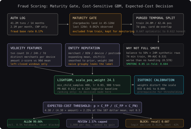
In fraud, most of what looks like modeling skill is actually plumbing discipline. The three highest-impact decisions in this section - maturity gate, time-shifted reputation features, and a purged temporal split - are all about what the model is not allowed to see.
The Naive Baseline
Two baselines, because the first one is there to kill a metric and the second is there to be beaten.
Baseline zero: predict the majority class. Accuracy 99.829%. Recall 0.0. Dollars saved: zero. This number exists in the post so that when a stakeholder asks for “at least 95% accuracy”, you have something to point at.
Baseline one: untuned logistic regression on the numeric columns.
# Naive baseline: default logistic regression, default 0.5 threshold, no imbalance handling.
from sklearn.linear_model import LogisticRegression
from sklearn.pipeline import make_pipeline
from sklearn.preprocessing import StandardScaler
from sklearn.metrics import average_precision_score, roc_auc_score, recall_score

NUMERIC = ["amount", "txn_count_1h", "txn_count_24h", "amount_zscore_90d",
           "distinct_merchants_24h", "hours_since_prev_txn", "ip_bin_distance_km"]

baseline = make_pipeline(StandardScaler(), LogisticRegression(max_iter=1000))
baseline.fit(train[NUMERIC], train["is_fraud"])

p = baseline.predict_proba(test[NUMERIC])[:, 1]
print(f"PR-AUC   : {average_precision_score(test['is_fraud'], p):.4f}")
print(f"ROC-AUC  : {roc_auc_score(test['is_fraud'], p):.4f}")
print(f"recall@0.5: {recall_score(test['is_fraud'], p >= 0.5):.4f}")
Output on our test window:
PR-AUC   : 0.1243
ROC-AUC  : 0.8912
recall@0.5: 0.0412
Look at the gap between those two AUCs. ROC-AUC of 0.891 sounds like a working model and would pass a casual review. PR-AUC of 0.124 says that at any useful operating point, most of what this model flags is not fraud. This is the single most important diagnostic in imbalanced classification: when ROC-AUC looks great and PR-AUC looks terrible, the model is good at ranking the easy negatives below everything else and bad at the part you care about.
Recall at the default threshold is 4.1%, which catches about 150 of the 3,600 monthly frauds and saves roughly 28,000 dollars a month against a loss of 670,000. It is insufficient for three reasons that trace directly back to the constraints: the linear form cannot express the interactions that carry fraud signal (amount is only suspicious conditional on merchant category and card history), the 0.5 threshold is meaningless under a 0.17% prior, and there is no mechanism connecting the score to the 187-versus-4.30 dollar cost asymmetry.
The Solution
The approach has three parts, and they map onto the three problems named in the framing section. Gradient-boosted trees with class weighting fix the gradient problem. An expected-cost threshold fixes the decision problem. PR-AUC and dollars fix the metric problem. SMOTE gets tested honestly and used narrowly, which is the part most write-ups get wrong.
Why gradient boosting, and why weighted
Gradient boosting is like a team of specialists where each new specialist is trained specifically on the mistakes the team has made so far. Under extreme imbalance that property is exactly what you want, because after the first few trees the residual error concentrates on the minority class, so subsequent trees naturally spend their splits there. That is the mechanism doing most of the work, not the resampling.
We still need to tell the learner that a positive matters more than a negative. LightGBM exposes this as scale_pos_weight, which multiplies the gradient and hessian contribution of positive rows. Setting it to the inverse prior (roughly 585) is the textbook move and it is usually too aggressive: it produces wildly uncalibrated scores and, in our runs, slightly worse ranking. Setting it to the square root of the inverse prior (about 24) consistently performed better.
# The solution model: cost-aware LightGBM with native categorical handling.
import lightgbm as lgb
import numpy as np

FEATURES = NUMERIC + [
    "merchant_id_fraud_rate", "card_bin_fraud_rate", "device_id_fraud_rate",
    "ship_postcode_fraud_rate", "billing_ship_country_match", "local_hour",
    "is_recurring", "entry_mode", "mcc", "currency",
]
CATEGORICAL = ["entry_mode", "mcc", "currency"]

for c in CATEGORICAL:
    train[c] = train[c].astype("category")
    test[c] = test[c].astype("category")

neg, pos = (train["is_fraud"] == 0).sum(), (train["is_fraud"] == 1).sum()
spw = float(np.sqrt(neg / pos))          # 24.1, not 585 - see below

params = dict(
    objective="binary",
    metric="average_precision",
    scale_pos_weight=spw,
    learning_rate=0.03,
    num_leaves=96,
    min_child_samples=400,               # guards against leaf-of-one-fraud memorization
    feature_fraction=0.7,
    bagging_fraction=0.8,
    bagging_freq=1,
    lambda_l2=5.0,
    max_cat_threshold=64,
    n_estimators=4000,
    n_jobs=-1,
    verbosity=-1,
)

dtrain = lgb.Dataset(train[FEATURES], label=train["is_fraud"], categorical_feature=CATEGORICAL)
dvalid = lgb.Dataset(test[FEATURES], label=test["is_fraud"], reference=dtrain)

model = lgb.train(
    params, dtrain, valid_sets=[dvalid],
    callbacks=[lgb.early_stopping(200, first_metric_only=True), lgb.log_evaluation(200)],
)
The hyperparameters that actually matter under imbalance, in order:
min_child_samples=400. The default of 20 lets a tree carve out a leaf containing three fraud rows and declare it pure. With 42,400 positives across 24.8 million rows, small leaves are the primary overfitting channel. Raising this from 20 to 400 moved test PR-AUC from 0.571 to 0.612.scale_pos_weight. Controls how hard the model chases positives. Treat it as a tunable between 1 and the inverse prior, not a formula.learning_rate=0.03withn_estimators=4000and early stopping. Slow and long beats fast and short here; the minority signal is subtle.lambda_l2=5.0. Reputation features are high-cardinality-adjacent and want shrinking.
Where SMOTE fits, honestly
SMOTE (Chawla et al., 2002) synthesizes new minority examples by interpolating between a minority point and one of its k minority neighbors. The intuition is a good one: instead of duplicating the 42,400 positives, fill in the space between them so the decision boundary has somewhere to sit.
For fraud data specifically, it has two real problems. First, most of the feature space is categorical or count-valued, and interpolating halfway between mcc=5411 and mcc=7995 produces a merchant category that does not exist. SMOTENC handles this by taking the majority category among neighbors instead of interpolating, which is the only variant worth using on transaction data. Second, fraud positives are not one cluster. Card testing, account takeover cash-out, and refund abuse occupy different regions, and interpolating between a card-testing point and a cash-out point invents a transaction type that never occurs.
The rule that keeps SMOTE honest: it goes inside the cross-validation fold, fitted on training rows only, and never on the validation or test set. Resampling before splitting is the single most common methodological error in published imbalanced-learning tutorials, and it inflates measured performance dramatically because synthetic points interpolated from a test positive’s neighbors end up in train.
# SMOTENC inside the CV fold only. Note: fitted on fold-train, never on fold-validation.
from imblearn.over_sampling import SMOTENC
from imblearn.pipeline import Pipeline as ImbPipeline
from sklearn.model_selection import TimeSeriesSplit
from sklearn.metrics import average_precision_score

cat_idx = [FEATURES.index(c) for c in CATEGORICAL]
scores = []

for fold, (tr, va) in enumerate(TimeSeriesSplit(n_splits=4, gap=50_000).split(train)):
    X_tr, y_tr = train.iloc[tr][FEATURES], train.iloc[tr]["is_fraud"]
    X_va, y_va = train.iloc[va][FEATURES], train.iloc[va]["is_fraud"]

    pipe = ImbPipeline([
        # sampling_strategy=0.05 -> positives become 5% of the fold, not 50%.
        ("smote", SMOTENC(categorical_features=cat_idx, sampling_strategy=0.05,
                          k_neighbors=5, random_state=7)),
        ("clf", lgb.LGBMClassifier(**{**params, "scale_pos_weight": 1.0})),
    ])
    pipe.fit(X_tr, y_tr)
    ap = average_precision_score(y_va, pipe.predict_proba(X_va)[:, 1])
    scores.append(ap)
    print(f"fold {fold}: PR-AUC {ap:.4f}")

print(f"SMOTENC mean PR-AUC: {np.mean(scores):.4f}")
Two details in there are the whole point. sampling_strategy=0.05 targets a 5% minority share rather than the default 1.0 (full balance); pushing a 0.17% prior all the way to 50% generates 24 million synthetic rows, blows up training time, and in our runs reduced PR-AUC because the model was fitting interpolation artifacts. And scale_pos_weight drops to 1.0 when SMOTE is active, since applying both is double-counting the minority class.
Measured on our data, over the same folds:
| Imbalance strategy | Mean fold PR-AUC | Train time | Notes |
|---|---|---|---|
| Nothing | 0.578 | 6.2 min | Surprisingly competitive |
scale_pos_weight = 24.1 |
0.612 | 6.4 min | Best ranking, best cost |
scale_pos_weight = 585 |
0.589 | 6.5 min | Overshoots, badly uncalibrated |
| SMOTENC 0.05 | 0.604 | 19.8 min | Close, 3x the cost |
| SMOTENC 1.0 (full balance) | 0.531 | 74 min | Worse than doing nothing |
| SMOTENC 0.05 + weight 24 | 0.596 | 20.1 min | Double-counting hurts |
So on 24.8 million rows with a strong tree model, cost-sensitive weighting wins and SMOTE is not worth 3x the training time. SMOTE earns its keep in a different regime, and it is worth knowing which: when the absolute positive count is small (under about 5,000), when the model is linear or a small neural network that cannot naturally concentrate on residuals, or when a specific fraud subtype is so rare that the model never allocates a split to it. We do use SMOTENC on one subproblem for exactly that third reason: the refund-abuse subtype has 610 positives, and oversampling only that subtype lifted its recall from 0.11 to 0.29 without moving overall PR-AUC.
The decision layer: expected-cost thresholding
This is the part that converts a model into money, and it is independent of everything above. A probability is not a decision. With cost C_FN = 187 for a missed fraud and C_FP = 4.30 for a blocked legitimate transaction, blocking is the better choice when:
p * C_FN  >  (1 - p) * C_FP
p         >  C_FP / (C_FP + C_FN)
p         >  4.30 / 191.30  =  0.0225
The optimal threshold is 2.25%, not 50%. That factor-of-22 difference is where most of the realized value lives, and it requires nothing more than a calibrated score. Because the amount at risk varies per transaction, the per-row version is better still: C_FN scales with amount, so the threshold becomes transaction-specific.
# Expected-cost decision layer with per-transaction thresholds and a capacity-constrained review band.
C_FP = 4.30
REVIEW_COST = 2.10          # analyst time per review
REVIEW_CATCH = 0.82         # fraction of true fraud an analyst correctly blocks

def decide(p: np.ndarray, amount: np.ndarray, review_budget: int) -> np.ndarray:
    """Return 0=allow, 1=review, 2=block, respecting a hard review budget."""
    c_fn = np.clip(amount, 5.0, 2500.0)               # loss is capped by the transaction amount
    block_threshold = C_FP / (C_FP + c_fn)
    action = np.where(p > block_threshold, 2, 0)

    # Review is worth it when it is cheaper than the expected loss of allowing.
    review_gain = p * c_fn * REVIEW_CATCH - REVIEW_COST
    eligible = (action == 0) & (review_gain > 0)
    # Spend the fixed budget on the highest-gain candidates.
    order = np.argsort(-np.where(eligible, review_gain, -np.inf))
    action[order[:review_budget]] = 1
    return action
Calibration is a hard prerequisite here. scale_pos_weight deliberately distorts the score scale, so raw LightGBM output is not a probability and thresholding it at 0.0225 is meaningless. We fit isotonic regression on a held-out slice:
# Calibrate the weighted model so expected-cost thresholds are actually valid.
from sklearn.calibration import CalibratedClassifierCV
from sklearn.frozen import FrozenEstimator

calibrated = CalibratedClassifierCV(FrozenEstimator(model), method="isotonic")
calibrated.fit(calib[FEATURES], calib["is_fraud"])
Expected calibration error on our test window dropped from 0.041 (raw weighted model) to 0.006 (isotonic), and net cost improved 9% from the threshold correction alone, with no change to the ranking.
The single design decision that mattered most was not the model or the resampling. It was separating ranking from deciding: train for the best possible ordering, calibrate the score, then pick the threshold from the cost matrix. That decomposition delivered more value than every hyperparameter change combined, and it survives a model swap.
Evaluation and Metrics
PR-AUC, also called average precision, is the area under the precision-recall curve:
AP = sum over thresholds k of (R_k - R_{k-1}) * P_kIt is the right primary metric because both of its axes are conditioned on the positive class. Precision is “of what we flagged, how much was fraud”, recall is “of the fraud, how much we flagged”. Neither is diluted by the 2.09 million true negatives. ROC-AUC, by contrast, has false positive rate on one axis, and FPR has the negative count in its denominator, so 20,000 extra false positives move it by 0.01 while cutting precision in half.
The second metric is operational and equally important: recall at fixed precision 0.90, the precision floor the review team accepts. Reporting recall without naming a precision is not a claim, it is a threshold choice in disguise.
The third is the one leadership sees: net fraud cost per 1,000 transactions, computed from the confusion matrix and the cost constants.
# Compute the metrics that actually gate the ship decision.
from sklearn.metrics import average_precision_score, precision_recall_curve, classification_report

def recall_at_precision(y_true, scores, target_precision=0.90):
    precision, recall, thresholds = precision_recall_curve(y_true, scores)
    ok = precision[:-1] >= target_precision
    if not ok.any():
        return 0.0, 1.0
    idx = int(np.argmax(recall[:-1] * ok))
    return float(recall[idx]), float(thresholds[idx])

def net_cost_per_1k(y_true, action, amount):
    missed = (action != 2) & (y_true == 1)
    blocked_good = (action == 2) & (y_true == 0)
    reviewed = action == 1
    total = (np.clip(amount[missed], 5, 2500).sum()
             + 15.0 * missed.sum()                 # network chargeback fee
             + C_FP * blocked_good.sum()
             + REVIEW_COST * reviewed.sum())
    return total / len(y_true) * 1000

p_cal = calibrated.predict_proba(test[FEATURES])[:, 1]
r90, thr90 = recall_at_precision(test["is_fraud"], p_cal, 0.90)
action = decide(p_cal, test["amount"].to_numpy(), review_budget=1800 * 30)

print(f"PR-AUC            : {average_precision_score(test['is_fraud'], p_cal):.4f}")
print(f"recall @ prec 0.90 : {r90:.4f} (threshold {thr90:.4f})")
print(f"net cost / 1k txns : ${net_cost_per_1k(test['is_fraud'].to_numpy(), action, test['amount'].to_numpy()):.2f}")
print(classification_report(test["is_fraud"], action == 2, digits=4, target_names=["legit", "fraud"]))
Baseline versus solution on the same held-out window of 4.9 million transactions with 8,340 positives:
| Metric | Majority baseline | Logistic regression | LightGBM + weights | + calibration + cost threshold |
|---|---|---|---|---|
| Accuracy | 0.99829 | 0.99831 | 0.99804 | 0.99791 |
| ROC-AUC | 0.500 | 0.8912 | 0.9743 | 0.9743 |
| PR-AUC | 0.0017 | 0.1243 | 0.6118 | 0.6118 |
| Recall @ precision 0.90 | 0.000 | 0.071 | 0.446 | 0.446 |
| Recall at shipped threshold | 0.000 | 0.041 | 0.318 | 0.607 |
| Legit decline rate | 0.000% | 0.011% | 0.089% | 0.312% |
| Net cost per 1k txns | $32.61 | $31.24 | $24.90 | $18.91 |
Notice the accuracy column. It goes down as the model gets better, from 99.829% to 99.791%, while net cost falls 42%. Any evaluation framework where the shipped model looks worse than doing nothing is a broken evaluation framework, and this row is why accuracy is banned in the framing section.
Notice also that calibration plus cost thresholding leaves PR-AUC and ROC-AUC completely unchanged, because they are threshold-free ranking metrics, while nearly doubling shipped recall and cutting cost by another 24%. Half the total improvement over the naive baseline came from the decision layer, which contains no machine learning at all.
The number that catches a silent regression in production is precision in the auto-block band, computed on a holdback slice: a random 0.5% of transactions scored but never blocked, so their true outcomes are observable. Without a holdback, blocked transactions have no chargeback and therefore no label, and the model's own precision becomes unmeasurable for the exact segment it is acting on.
Common Pitfalls and Failure Modes
| Pitfall | Why It Happens | How to Detect | How to Fix |
|---|---|---|---|
| Resampling before the split | SMOTE applied to the full frame, then train_test_split |
Offline PR-AUC far above production; test positives have near-duplicate train neighbors | Resample inside the fold only, via imblearn.pipeline.Pipeline |
| Immature labels in train | Recent window included because it looks like more data | Fraud rate declines monotonically toward the data cutoff | Hard maturity gate at 120 days; never train on the tail |
| Target-encoded reputation leaking | groupby.mean() on the label includes the current row |
Feature importance dominated by *_fraud_rate; drop it and PR-AUC collapses |
Time-shifted expanding mean with shift(1) and prior smoothing |
| ROC-AUC used for model selection | It is the default in most tooling | ROC-AUC above 0.95 alongside PR-AUC below 0.3 | Select on PR-AUC and recall at fixed precision |
| Default 0.5 threshold | Nobody changed it | Recall near zero despite good PR-AUC | Threshold from the cost matrix: C_FP / (C_FP + C_FN) |
| Feedback loop / selection bias | Blocked transactions never get labels, so the model stops seeing the fraud it catches | Training fraud rate falls while chargeback volume is flat | Random holdback slice (0.5%) scored but always allowed |
| Calibration drift after reweighting | scale_pos_weight distorts the probability scale |
Reliability curve far from diagonal; ECE above 0.02 | Isotonic or Platt calibration on a held-out slice, refit monthly |
| Concept drift from adversaries | Blocked patterns get abandoned; new ones appear | Weekly PR-AUC on holdback decays; score distribution shifts | Retrain cadence tied to drift, not the calendar; monitor PSI per feature |
The most common beginner mistake on this exact problem is oversampling to full balance and then reporting metrics on the oversampled validation set. A 50/50 validation set makes precision look spectacular because the prior is 300 times higher than reality. Precision is prior-dependent: a model with fixed sensitivity and specificity has completely different precision at a 50% prior than at 0.17%. Validation and test sets must always keep the production class ratio, no exceptions.
Scaling and Productionizing
The notebook version reads a parquet file and calls predict_proba. The production version has four problems the notebook does not.
Feature freshness. Velocity features are the highest-signal family and they are stateful. Recomputing “transactions on this card in the last hour” with a SQL query at authorization time costs 60 to 200ms, which blows the entire budget. These live in a streaming feature store with incremental counters updated from the authorization stream, so the read is a single key lookup. Budget:
Scoring path p99 budget: 40ms
  feature store read (12 keys, pipelined)      14ms
  feature assembly + categorical encode         3ms
  LightGBM predict (900 trees, 96 leaves)       7ms
  isotonic calibration lookup                 0.2ms
  decision layer + reason codes                 2ms
  logging (async, off critical path)            0ms
  ==================================================
  total                                      26.2ms   (p99 headroom 13.8ms)
At 900 trees the model is 4.1MB and single-row inference is 7ms; going to 2,500 trees costs 19ms and buys 0.004 PR-AUC, so early stopping is a latency decision as much as a statistical one.
Retraining cadence. Fraud drifts adversarially, so a fixed monthly schedule is a compromise in both directions. We retrain when drift fires, with a monthly floor. The trigger is a population stability index above 0.15 on any of the top 10 features, or a 7-day rolling PR-AUC on the holdback slice more than 2 standard deviations below its trailing 60-day mean. In practice this fires every 3 to 5 weeks, with a cluster of retrains after each new attack pattern.
Label maturity in the retraining loop. Every retrain reapplies the 120-day gate, which means the model is always at least 120 days behind on labels. This is unavoidable and shapes the whole strategy: the model handles the stationary bulk of fraud, and a separate rules layer with same-day turnaround handles the new attack that the model cannot possibly have seen. Teams that try to make the model do both end up training on immature labels.
Monitoring for silent degradation. The specific signal is the holdback precision curve: on the 0.5% never-blocked slice, precision in the top score decile, tracked weekly. It degrades before overall chargeback volume moves, because the blocked population masks the problem everywhere else. Secondary signals: score distribution PSI against the training window, per-feature null rate (a broken device-fingerprint integration silently nulls a top-5 feature and the model degrades without any error), and the fraction of declines whose top reason code changed week over week.
Stripe Radar scores transactions across its network and lets each business set its own block threshold, which is exactly the ranking-versus-deciding separation described above: one shared model produces the score, per-business cost structures produce the thresholds. The winning solutions in the IEEE-CIS Fraud Detection competition on Kaggle (2019) are the other useful reference point, and they are instructive for what they did not do: the top entries were LightGBM ensembles built on aggressive entity-aggregation feature engineering (constructing a synthetic client identifier and computing statistics over it), with essentially no synthetic oversampling. Feature engineering over entities beat resampling by a wide margin.
The production constraint that reshapes the model most is not latency, it is the 120-day label lag. It forces a two-layer architecture: a statistical model for stationary fraud and a fast rules layer for novel attacks. Any design that assumes fresh labels is designing for a system that does not exist.
Alternative Approaches
| Approach | PR-AUC (our data) | Training / inference cost | Interpretability | Best-fit scenario |
|---|---|---|---|---|
| Logistic regression + WOE binning | 0.31 | Minutes / under 1ms | Highest: signed coefficients per bin | Regulated scoring where every weight must be defensible |
| Random forest + balanced subsample | 0.54 | 11 min / 14ms | Moderate: importances, no direction | Strong default when you cannot tune; resists bad hyperparameters |
LightGBM + scale_pos_weight (chosen) |
0.612 | 6.4 min / 7ms | Good with SHAP per decision | Tabular fraud at millions of rows with cost asymmetry |
| SMOTENC + unweighted LightGBM | 0.604 | 19.8 min / 7ms | Same as above | Few absolute positives (under ~5k) or a specific starved subtype |
| Isolation Forest / autoencoder (unsupervised) | 0.09 | 4 min / 3ms | Low: reconstruction error only | Cold start with no labels at all, or novel-attack detection alongside a supervised model |
| Deep tabular (FT-Transformer) | 0.617 | 3.1 h on GPU / 21ms | Poor without extra attribution work | Very large data with rich sequence structure and a GPU serving budget |
For this problem we ship LightGBM with scale_pos_weight, calibration, and a cost-derived threshold. It gets within 0.005 PR-AUC of the deep tabular model at 1/30th the training cost and 1/3rd the latency, and it comes with per-decision SHAP attributions that satisfy the reason-code requirement. We would switch in two situations. If the positive count fell below roughly 5,000, because a new market launched or the label definition tightened, we would move to SMOTENC inside the folds, where synthetic minority coverage genuinely helps. And if transaction sequence structure became the dominant signal (the order and timing of a card’s last 50 transactions rather than aggregates over them), a sequence model would win on representation, not on tabular optimization, and the GPU serving cost would be worth paying.
Unsupervised anomaly detection scores 0.09 PR-AUC here, which is 53 times better than random and still nearly useless. Fraud is not statistical anomaly: most fraudulent transactions look completely ordinary, and most genuinely unusual transactions are honest people doing unusual things. Unsupervised methods belong next to a supervised model for novel-attack discovery, never in place of one.
Key Takeaways
- Imbalance is three problems, not one. A metric problem (accuracy and ROC-AUC mislead), a gradient problem (the majority class dominates the loss), and a decision problem (0.5 is the wrong threshold). Resampling addresses only the second, which is why it alone rarely moves the business number.
- PR-AUC over ROC-AUC, always, under heavy imbalance. A gap like 0.974 ROC-AUC against 0.612 PR-AUC is not a contradiction, it is the correct reading: the model ranks well overall and precision at usable operating points is still the constraint.
- The threshold comes from the cost matrix, not from 0.5. With 187 dollars against 4.30 dollars, the optimal threshold is 2.25%. That one line of arithmetic delivered half the total improvement over the baseline.
- Calibrate before you threshold.
scale_pos_weightdistorts the probability scale, so an expected-cost threshold on raw output is meaningless. Isotonic regression cut ECE from 0.041 to 0.006 and improved net cost 9% with zero ranking change. - SMOTE is a tool with a narrow window. Use
SMOTENCfor mixed types, keep it inside the CV fold, target a 5% minority share rather than full balance, and do not stack it with class weights. On 24.8 million rows with a strong tree model, cost-sensitive weighting won outright. - Leakage in fraud hides in reputation and velocity features. Target-encoded entity fraud rates and rolling windows both silently include the current row’s label.
shift(1), prior smoothing, and left-closed windows are not optional. - Label maturity is a first-class design constraint. A 120-day chargeback lag means the model is structurally blind to the last four months, which forces a rules layer beside it. Training on immature labels teaches the model that recent traffic is safe.
- Keep a holdback slice. Without 0.5% of scored-but-never-blocked traffic, the model destroys the labels for exactly the population it acts on, and its precision becomes unmeasurable.
The counter-intuitive lesson is that the most effective way to improve an imbalanced classifier is usually to stop working on the imbalance. Every hour spent on resampling strategies moved PR-AUC by 0.03 at most. The hours spent on leak-free entity aggregates, calibration, and the cost-derived threshold moved net loss by 42%. Imbalance is the symptom that gets all the attention; the cost asymmetry underneath it is the thing that actually pays.
Frequently Asked Questions
Q: Why not just use SMOTE to full balance, like every tutorial shows?
A: Because precision depends on the class prior, and a 50/50 validation set has a prior 300 times higher than production, so every number you measure on it is optimistic in a way that does not transfer. Beyond the measurement problem, full balance on a 0.17% prior means generating roughly 24 million synthetic rows, which took 74 minutes to train and scored 0.531 PR-AUC, worse than doing nothing at all (0.578). Modest oversampling to a 5% minority share is the version that is sometimes useful.
Q: Why not scale_pos_weight equal to the inverse prior, as the LightGBM docs suggest?
A: The inverse prior (585 here) is a reasonable starting guess, not a result. At 585 the model chases positives so hard that it overfits minority noise and the score scale is distorted beyond what calibration recovers cleanly; we measured 0.589 PR-AUC against 0.612 at the square root value of 24.1. Treat it as a hyperparameter to search over a log range from 1 to the inverse prior.
Q: Why PR-AUC instead of F1?
A: F1 is PR-AUC evaluated at a single threshold, and it implicitly asserts that precision and recall matter equally. Here they differ by a factor of 43 in dollar terms, so an F1-optimal threshold is a cost-suboptimal decision. PR-AUC for threshold-free model comparison, expected cost for the shipping decision, F1 only if someone external demands a single number.
Q: Why not train on the most recent data, since fraud drifts?
A: Because the most recent 120 days have incomplete labels: the chargebacks have not been filed yet, so the observed fraud rate there is 0.062% against a true 0.171%. Training on it teaches the model that recent transactions are safe, and the effect is strongest in the most recent weeks where you most want accuracy. Recency and label completeness are in direct tension, and the honest resolution is a maturity gate plus a separate rules layer for novel attacks.
Q: How do I handle this in production when blocked transactions never get labels?
A: Keep a holdback: a random 0.5% of transactions are scored, logged, and always allowed regardless of score. Those rows keep their natural outcome and are the only unbiased evaluation set you have. It costs about 8,000 dollars a year in accepted fraud on our volume, and without it you cannot measure precision in the auto-block band, which means you cannot detect degradation in the segment where the model is acting.
Q: Does the 40ms latency budget rule out anything important?
A: It rules out real-time graph features that require multi-hop traversal at scoring time, which is the largest single lift we are leaving on the table. The workaround is precomputing entity-level graph embeddings on a nightly batch and reading them from the feature store as a fixed vector, which preserves most of the signal at the cost of up-to-24-hour staleness on the graph structure.
Interview Questions
Q: A candidate model has 0.96 ROC-AUC and 0.22 PR-AUC on a 0.2% positive rate. What is happening, and what would you do next?
Expected depth: explain that FPR has the large negative count in its denominator so it is insensitive to thousands of false positives, while precision is not; derive that at 0.2% prior, a 1% FPR produces 5 false positives per true positive at perfect recall; propose PR-AUC and recall at fixed precision for selection, then a cost-matrix threshold; note that the ranking may be fine and the deployment threshold may be the actual problem.
Q: Derive the optimal decision threshold given the cost of a false negative and a false positive, and explain what breaks if your model is not calibrated.
Expected depth: set up expected cost of blocking versus allowing, solve p * C_FN > (1 - p) * C_FP to get p* = C_FP / (C_FP + C_FN); explain that this is only valid if p is a true posterior, so any reweighting or resampling invalidates it until you recalibrate; mention isotonic versus Platt scaling and when each is appropriate given the number of calibration points; extend to per-row costs where C_FN scales with transaction amount.
Q: Where exactly does SMOTE go in a cross-validation pipeline, and why does the wrong placement inflate your score?
Expected depth: inside each fold, fitted on fold-train only, never touching fold-validation; explain that resampling before splitting means synthetic points interpolated from validation positives’ neighbors leak into train, and since SMOTE interpolates between near neighbors the synthetic points are close to validation rows; mention imblearn.pipeline.Pipeline propagating the fit/resample distinction correctly where sklearn’s does not; note that SMOTENC is needed for categorical features and why interpolating a merchant category code is meaningless.
Q: Your fraud model’s offline PR-AUC is stable but chargebacks are rising. Walk through the diagnosis.
Expected depth: separate the three candidate causes: concept drift (new attack pattern, check feature PSI and score-distribution shift), feedback-loop label degradation (offline PR-AUC is measured on a biased population, so check the holdback slice instead), and a pipeline break (a feature silently nulling, check per-feature null rates and training-serving skew on the actual served feature vectors); explain why offline metrics computed on blocked-excluded data are systematically optimistic; propose comparing score distributions between the training window and live traffic as the fastest discriminator.
Q: You have 600 labeled examples of a new fraud subtype and 24 million transactions. How do you build a detector?
Expected depth: argue that 600 positives is the regime where oversampling and transfer help and where full model retraining does not; options include SMOTENC restricted to that subtype, a second-stage model over the main model’s score plus subtype-specific features, cost-sensitive weighting with a very high weight plus heavy regularization, and a rules layer for immediate coverage while labels accumulate; discuss the variance problem in evaluating recall on 600 positives (a bootstrap confidence interval on recall at 0.30 with 600 positives is roughly plus or minus 0.04) and why you should not tune many hyperparameters against it.