Build a Customer Lifetime Value Regression Model
classical-ml feature-engineering model-evaluation mlops View full code for this problem
ML Problem & Solution
Customer Lifetime Value Regression
62% of customers will spend nothing, and 1% will spend a fifth of your revenue
A non-subscription online retailer has 4.1 million customers who have bought at least once, and a marketing team with 62 million dollars a year to allocate across acquisition channels, retention campaigns, and a loyalty tier. Every one of those decisions needs the same number: how much net revenue will this customer generate over the next 24 months. The finance team wants it to sum correctly at the portfolio level. The growth team wants it to rank correctly so they can spend on the top decile. Those are not the same requirement, and a model that satisfies one usually fails the other.
Look at the target before choosing a model, because its shape is the whole problem. Over a 24 month horizon, 62% of existing customers spend exactly zero. Of the 38% who buy, the median spends 94 dollars and the 99th percentile spends 4,180 dollars. The top 1% of customers account for 22% of total forward revenue. So the target is a continuous variable with a huge point mass at zero and a long right tail, and neither half is a rounding error: the zeros are most of the customers and the tail is most of the money.
That shape breaks the reflexive approach immediately. Fit a gradient boosting regressor with the default squared-error objective and it will do something reasonable-looking and useless: because squared error is dominated by the largest residuals, the model spends its capacity trying to predict the 4,180 dollar customers, misses them anyway because they are genuinely rare, and in exchange predicts 180 dollars for a large population that will spend nothing. Root mean squared error looks acceptable. The decile ranking, which is what the growth team actually uses, is barely better than sorting by last year’s spend. The obvious fix, taking log1p of the target, makes the ranking better and quietly breaks the finance requirement, because the mean of a log-normal is not the exponential of the mean and back-transformed predictions undershoot the total by 30% or more.
The structure to hold onto is an insurance book. Most policyholders claim nothing in a year, a few claim a little, and a very few claim enormously. Actuaries stopped fitting squared error to that shape decades ago, and the distribution they reached for is exactly the one that fits this problem.
Given a customer’s transaction, engagement, and acquisition history up to a fixed cutoff date, predict their net revenue over the following 24 months, optimizing decile-level revenue capture and rank correlation, subject to the predicted portfolio total staying within 5% of actual.
Framing the Problem
This is regression on a zero-inflated, heavy-tailed, non-negative continuous target, evaluated jointly on ranking quality and on aggregate calibration. Calling it “regression” and moving on is how most CLV projects go wrong, because the zero inflation and the tail each demand a specific decision and the default objective makes both of them badly.
The target is clv_24m: the sum of net revenue across all orders placed in the 730 days after the cutoff date, where net revenue is gross merchandise value minus returns, minus the actual shipping cost, and minus payment processing fees. Two choices in that definition are load-bearing.
Net, not gross. Returns are 14.2% of gross revenue and are extremely unevenly distributed: the apparel category returns at 31% and the top spending decile returns at 24% against a 14% average. A gross revenue model systematically over-values exactly the customers marketing is about to spend the most on.
Returns need a settlement buffer. A return can be initiated up to 60 days after delivery, so an order placed on day 728 of the horizon does not have a final net value until roughly day 800. Computing the label at day 730 makes the last two months of the horizon look more profitable than they are. The fix is a label that is computed at cutoff plus 730 plus 60 days, which costs two extra months of data latency and is not optional.
Constraints
- Scoring cadence: monthly batch over 4.1 million customers. There is no latency constraint worth mentioning, which is unusual and means model complexity is nearly free here. What is not free is explainability to the marketing team.
- Aggregate calibration: the predicted portfolio total must land within 5% of actual, because the number feeds a finance forecast. This is what rules out an uncorrected log-transform model.
- Decile stability: a customer should not jump from decile 9 to decile 2 between two monthly scorings without a behavioural reason, because the loyalty tier is derived from the decile and customers notice being demoted.
- Horizon: fixed at 24 months. Shorter than the 18 month median repurchase interval in the home category would systematically undervalue it; much longer and the label is too stale to train on.
- Cold start is out of scope here: this model predicts for customers with at least one completed order. Predicting value for a not-yet-acquired visitor from ad-click context is a different problem with a different feature set.
Top-decile revenue capture: of all actual forward revenue, what share falls to customers the model put in its top predicted decile. A perfect model captures 61% here (the concentration ceiling given the actual revenue distribution), the RFM baseline captures 31%, and random captures 10%. It is the right headline metric because it maps directly onto how the output is used: marketing spends on a decile, not on a predicted dollar amount. RMSE is close to useless on this target, since it is dominated by a handful of customers nobody can predict individually and it improves when the model gives up and predicts the mean.
Guardrail metrics: predicted-to-actual total ratio at the portfolio level and within each decile, Spearman rank correlation, mean absolute error restricted to the top decile (where the dollars are), and decile transition churn month over month. Out of scope: the causal question of whether a retention campaign changes a customer’s value, which is an uplift modeling problem and cannot be answered by this model no matter how accurate it is.
The target distribution chooses the objective, not the other way round. A point mass at zero plus a heavy right tail is a compound Poisson-gamma distribution, which is exactly what the Tweedie family with a variance power between 1 and 2 describes. Once you see the target that way, "which loss function" stops being a hyperparameter search and becomes a modeling statement: purchases arrive as a Poisson process and each has a gamma-distributed value.
Data and Features
Four sources, joined at the customer level as of a fixed cutoff date.
| Source | Grain | Rows | Time range used |
|---|---|---|---|
orders |
order | 39M | full history, capped at 36 months before cutoff |
order_lines |
order x sku | 214M | same |
returns |
return | 5.1M | full history plus 60 day settlement |
sessions |
session | 1.6B | 12 months before cutoff |
customers |
customer | 4.1M | acquisition channel, first order date, region |
Window construction is the entire leakage story
Every CLV bug I have seen traces back to this diagram, so build it first and assert it in code.

There is a cutoff date. Everything strictly before it can be a feature. Everything in the 730 days after it is the label. Nothing may cross. The three ways it crosses in practice:
A feature computed from the full table. total_orders_lifetime computed against the whole orders table includes orders placed after the cutoff. This one is so easy to write that it appears in most first drafts, and it takes validation Spearman from a plausible 0.68 to an implausible 0.91, which is the tell.
Tenure-confounded aggregates. A customer acquired 34 months before cutoff has 34 months of feature history; one acquired 2 months before has 2 months. An unnormalized orders_in_feature_window therefore encodes tenure, and tenure correlates with forward value for a reason that will not hold next year (it is a function of when the company was running which acquisition campaign). Every count feature needs a rate twin: orders_per_active_month alongside orders_count.
Survivorship in the customer list. If the customer table is filtered to customers who still exist at scoring time, anyone who requested deletion, hard-bounced, or was flagged fraudulent inside the horizon is silently absent, and those are disproportionately zero-value customers. The population must be frozen as of the cutoff and carried forward whatever happens to it.
# Window construction with the assertions that make leakage a build failure
# rather than a review finding. Run this before any feature code.
from dataclasses import dataclass
import pandas as pd


@dataclass(frozen=True)
class Windows:
    cutoff: pd.Timestamp
    feature_months: int = 36
    horizon_days: int = 730
    settlement_days: int = 60      # returns can be initiated 60 days post delivery

    @property
    def feature_start(self) -> pd.Timestamp:
        return self.cutoff - pd.DateOffset(months=self.feature_months)

    @property
    def horizon_end(self) -> pd.Timestamp:
        return self.cutoff + pd.Timedelta(days=self.horizon_days)

    @property
    def label_final_on(self) -> pd.Timestamp:
        # The date the label stops changing. Train only on cohorts past this.
        return self.horizon_end + pd.Timedelta(days=self.settlement_days)


def slice_features(orders: pd.DataFrame, w: Windows) -> pd.DataFrame:
    frame = orders[(orders["order_ts"] >= w.feature_start)
                   & (orders["order_ts"] < w.cutoff)]
    if frame["order_ts"].max() >= w.cutoff:
        raise AssertionError("feature slice contains post-cutoff orders")
    return frame


def slice_horizon(orders: pd.DataFrame, w: Windows) -> pd.DataFrame:
    frame = orders[(orders["order_ts"] >= w.cutoff)
                   & (orders["order_ts"] < w.horizon_end)]
    if frame["order_ts"].min() < w.cutoff:
        raise AssertionError("horizon slice contains pre-cutoff orders")
    return frame


def assert_label_is_settled(w: Windows, data_as_of: pd.Timestamp) -> None:
    if data_as_of < w.label_final_on:
        raise AssertionError(
            f"labels for cutoff {w.cutoff.date()} are not final until "
            f"{w.label_final_on.date()}, data only runs to {data_as_of.date()}. "
            "Training now treats un-returned orders as kept revenue."
        )
The label
# Net forward revenue per customer over the horizon, with returns settled.
# Customers with no forward orders get an explicit 0.0, not a missing value:
# they are 62% of the population and they are the signal, not absence of it.
import numpy as np
import pandas as pd


def build_label(population: pd.DataFrame, orders: pd.DataFrame,
                returns: pd.DataFrame, w: Windows) -> pd.DataFrame:
    horizon = slice_horizon(orders, w)

    # Returns are matched to their order, and counted whenever the return is
    # initiated, including after horizon_end but before label_final_on.
    settled = returns[returns["return_ts"] < w.label_final_on]
    refunds = (settled.merge(horizon[["order_id", "customer_id"]],
                             on="order_id", how="inner")
               .groupby("customer_id")["refund_amount"].sum())

    gross = horizon.groupby("customer_id")["gmv"].sum()
    ship = horizon.groupby("customer_id")["shipping_cost"].sum()
    fees = horizon.groupby("customer_id")["payment_fees"].sum()

    out = population[["customer_id"]].copy()
    for name, series in (("gross", gross), ("refunds", refunds),
                         ("ship", ship), ("fees", fees)):
        out[name] = out["customer_id"].map(series).fillna(0.0)

    out["clv_24m"] = (out["gross"] - out["refunds"] - out["ship"]
                      - out["fees"]).clip(lower=0.0)
    out["purchased"] = (out["clv_24m"] > 0).astype(np.int8)
    return out
Features that actually carry signal
We run 74 features. The ones that matter cluster into four groups, and the ordering by permutation importance on the Tweedie model is stable across cutoffs.
# RFM core plus the trend and diversity features that beat plain RFM.
# Every count feature has a rate twin so the model is not reading tenure.
def build_features(orders: pd.DataFrame, lines: pd.DataFrame,
                   sessions: pd.DataFrame, population: pd.DataFrame,
                   w: Windows) -> pd.DataFrame:
    hist = slice_features(orders, w)
    feats = population[["customer_id", "acquisition_channel",
                        "first_order_ts", "region"]].copy()

    agg = hist.groupby("customer_id").agg(
        orders_count=("order_id", "nunique"),
        gross_total=("gmv", "sum"),
        gross_mean=("gmv", "mean"),
        gross_max=("gmv", "max"),
        gross_std=("gmv", "std"),
        last_order_ts=("order_ts", "max"),
        first_seen_ts=("order_ts", "min"),
    )
    feats = feats.merge(agg, on="customer_id", how="left")

    # Recency and tenure, both in days, both measured from the cutoff.
    feats["recency_days"] = (w.cutoff - feats["last_order_ts"]).dt.days
    feats["tenure_days"] = (w.cutoff - feats["first_order_ts"]).dt.days
    feats["active_months"] = (feats["tenure_days"] / 30.44).clip(lower=1.0)

    # Rate twins: this is what stops count features encoding tenure.
    feats["orders_per_month"] = feats["orders_count"] / feats["active_months"]
    feats["gross_per_month"] = feats["gross_total"] / feats["active_months"]

    # Trend: last 6 months of spend against the 6 before it. The single
    # strongest non-RFM feature, and the one plain RFM cannot express.
    recent = _window_sum(hist, w.cutoff, 0, 182)
    prior = _window_sum(hist, w.cutoff, 182, 365)
    feats["spend_recent_182d"] = feats["customer_id"].map(recent).fillna(0.0)
    feats["spend_prior_182d"] = feats["customer_id"].map(prior).fillna(0.0)
    feats["spend_trend"] = ((feats["spend_recent_182d"] + 1.0)
                            / (feats["spend_prior_182d"] + 1.0))

    # Inter-purchase regularity: a customer who buys every 40 days plus or
    # minus 5 is worth far more than one who bought 6 times in one week.
    gaps = (hist.sort_values("order_ts").groupby("customer_id")["order_ts"]
            .diff().dt.days)
    gap_stats = gaps.groupby(hist["customer_id"]).agg(["mean", "std"])
    feats["ipt_mean"] = feats["customer_id"].map(gap_stats["mean"])
    feats["ipt_cv"] = feats["customer_id"].map(
        gap_stats["std"] / gap_stats["mean"].clip(lower=1.0))

    # Category breadth: customers who bought across 3+ categories churn less.
    breadth = (lines[lines["order_id"].isin(set(hist["order_id"]))]
               .groupby("customer_id")["category"].nunique())
    feats["categories_bought"] = feats["customer_id"].map(breadth).fillna(0)

    # Return propensity: the feature that keeps the model from over-valuing
    # the apparel-heavy top decile, which returns at 24% against a 14% average.
    feats["return_rate_hist"] = _historical_return_rate(hist, w)

    # Engagement, from sessions only inside the feature window.
    sess = sessions[(sessions["session_ts"] >= w.cutoff
                     - pd.Timedelta(days=365))
                    & (sessions["session_ts"] < w.cutoff)]
    eng = sess.groupby("customer_id").agg(
        sessions_365d=("session_id", "nunique"),
        last_session_ts=("session_ts", "max"))
    feats = feats.merge(eng, on="customer_id", how="left")
    feats["session_recency_days"] = (
        w.cutoff - feats["last_session_ts"]).dt.days
    # Browsing without buying is the strongest early warning of a lapsing
    # customer, and the strongest signal of a returning one.
    feats["sessions_per_order"] = (feats["sessions_365d"].fillna(0.0)
                                   / feats["orders_count"].clip(lower=1))

    return feats.drop(columns=["last_order_ts", "first_seen_ts",
                               "last_session_ts", "first_order_ts"])
Top features by permutation importance on top-decile capture: spend_recent_182d, recency_days, orders_per_month, spend_trend, ipt_cv, gross_mean, sessions_per_order, categories_bought, return_rate_hist, acquisition_channel. Notice that four of the top eight are things plain RFM cannot express, and two of them (spend_trend, sessions_per_order) are ratios of quantities RFM already has.
The split
A random split is wrong here for a reason that is worth being precise about, because it is not the usual one. The features and labels are already separated in time by construction, so a random split does not leak the future into the past. What it does leak is the macro period: all training and validation customers experience the same 24 months of promotions, stockouts, and demand conditions, so the model learns that period’s repurchase rates as if they were properties of customers. Deployed against a different macro period, aggregate calibration drifts even though the ranking holds up.
# Two cutoffs, separated by a full horizon. Train on the older, validate on the
# newer. This is the only split that measures what happens when the macro
# period changes, which is the failure the monthly retrain has to survive.
def cohort_split(orders, returns, sessions, customers,
                 train_cutoff: pd.Timestamp, test_cutoff: pd.Timestamp,
                 data_as_of: pd.Timestamp):
    train_w = Windows(cutoff=train_cutoff)
    test_w = Windows(cutoff=test_cutoff)
    assert_label_is_settled(train_w, data_as_of)
    assert_label_is_settled(test_w, data_as_of)

    parts = {}
    for name, w in (("train", train_w), ("test", test_w)):
        # Population frozen as of the cutoff: no survivorship filtering.
        population = customers[customers["first_order_ts"] < w.cutoff]
        x = build_features(orders, lines, sessions, population, w)
        y = build_label(population, orders, returns, w)
        parts[name] = x.merge(y, on="customer_id", validate="one_to_one")
return parts["train"], parts["test"]Dropping customers whose label is zero, on the theory that they are "inactive" and not really part of the population. This is the most damaging single mistake available on this problem. Those customers are 62% of the population, the model's entire job at the bottom of the distribution is to identify them, and removing them turns a CLV model into a conditional-value model whose predictions are 2.6x too high for everyone. If the business genuinely wants conditional value, model it explicitly as the second stage of a two-part model and keep the first stage.
The Naive Baseline
Two baselines, both of which are actually deployed at real companies, and both with real numbers on a held-out cutoff of 1.24 million customers whose actual 24 month net revenue totals 214.6 million dollars.
# Baseline 1: RFM scoring. Rank customers on recency, frequency and monetary
# quintiles, sum the scores, and treat the score as value. Still the most
# widely deployed CLV method in retail.
# Baseline 2: naive extrapolation. Assume the next 24 months look like the last
# 24 months, scaled by a survival haircut.
import numpy as np
import pandas as pd


def rfm_score(feats: pd.DataFrame) -> pd.DataFrame:
    out = feats[["customer_id"]].copy()
    # Recency reversed: more recent is better.
    out["r"] = pd.qcut(-feats["recency_days"].rank(method="first"),
                       5, labels=[1, 2, 3, 4, 5]).astype(int)
    out["f"] = pd.qcut(feats["orders_count"].rank(method="first"),
                       5, labels=[1, 2, 3, 4, 5]).astype(int)
    out["m"] = pd.qcut(feats["gross_mean"].fillna(0.0).rank(method="first"),
                       5, labels=[1, 2, 3, 4, 5]).astype(int)
    out["rfm"] = out["r"] + out["f"] + out["m"]
    return out


def rfm_value(feats: pd.DataFrame, train_labels: pd.DataFrame) -> np.ndarray:
    """Turn the RFM score into dollars by averaging observed CLV per score.

    Without this step RFM is a 3-to-15 integer and cannot be compared against a
    regression on any calibration metric.
    """
    scored = rfm_score(feats).merge(train_labels, on="customer_id")
    lookup = scored.groupby("rfm")["clv_24m"].mean()
    return rfm_score(feats)["rfm"].map(lookup).fillna(
        train_labels["clv_24m"].mean()).to_numpy()


def naive_extrapolation(feats: pd.DataFrame, survival: float = 0.38) -> np.ndarray:
    """Last 24 months of spend, haircut by the observed repurchase rate."""
    trailing = feats["gross_per_month"].fillna(0.0) * 24.0
    return (trailing * survival).to_numpy()
Measured on the held-out cutoff:
| Baseline | Spearman | Top-decile revenue capture | Total ratio | RMSE |
|---|---|---|---|---|
| Predict the mean (52.14 dollars) | 0.000 | 10.0% | 1.000 | 386.1 |
| Naive extrapolation | 0.372 | 28.4% | 1.212 | 431.7 |
| RFM quintile scoring | 0.412 | 31.1% | 1.004 | 379.4 |
Note the second row carefully. Naive extrapolation has a worse RMSE than predicting the mean, while being obviously more informative. That is the first sign that RMSE is the wrong metric on this target: a model that takes real risk on the tail is punished for the times it is wrong more than it is rewarded for the times it is right.
RFM is the baseline to beat, and its weaknesses are specific. It is a rank statistic, so it cannot represent magnitude at all: a customer at the 99.9th percentile of spend and one at the 85th both land in quintile 5. It uses three features, so it cannot see the trend, the regularity, the breadth, or the return propensity that turn out to matter. And its quintile boundaries are recomputed each scoring run, which means customers get demoted for no reason other than that other customers moved, which is exactly the decile churn the loyalty tier cannot tolerate.
The Solution
Fit LightGBM with a Tweedie objective, tweedie_variance_power = 1.5, directly on the raw dollar target, with no log transform and no dropping of zeros. Then check it against a two-part model and a zero-inflated lognormal, because on this problem the choice between the three is genuinely close and depends on what the output is for.
Why Tweedie is the right objective
The Tweedie family interpolates between distributions by a variance power p, where Var(Y) = phi * E(Y)^p. At p = 1 it is Poisson, at p = 2 it is gamma, and for 1 < p < 2 it is a compound Poisson-gamma: a Poisson-distributed number of events, each with a gamma-distributed size. Write down what generates CLV and you get exactly that. A customer makes some number of purchases in 24 months, which is a count process, and each purchase has a positive continuous value with a right-skewed distribution.
The compound Poisson-gamma has an atom at zero, with mass equal to the probability of zero events, and a smooth positive density above it. That is the target’s shape, not an approximation of it. Squared error, by contrast, corresponds to a Gaussian likelihood, which places zero probability mass at any single point and assumes constant variance, both of which are false here by a wide margin.
Analogy: squared error asks “how far off is my guess”, which treats a 20 dollar error on a 0 dollar customer and a 20 dollar error on a 4,000 dollar customer as identical mistakes. Tweedie asks “how surprising is this outcome under my predicted rate”, which treats them as very different, because 20 dollars is infinitely surprising for a customer predicted to spend nothing and unremarkable for one predicted to spend thousands.
# The solution: LightGBM with a Tweedie objective on the raw dollar target.
# No log transform, no dropped zeros, no two-stage plumbing.
import lightgbm as lgb
import numpy as np
import pandas as pd

CATEGORICAL = ["acquisition_channel", "region"]

PARAMS = {
    "objective": "tweedie",
    # 1.5 sits mid-family: enough zero mass for a 62% zero rate, enough
    # gamma tail for a 99th percentile at 44x the median. Tuned on a grid of
    # [1.1, 1.3, 1.5, 1.7, 1.9]; 1.5 and 1.7 are within noise of each other.
    "tweedie_variance_power": 1.5,
    "metric": "tweedie",
    "learning_rate": 0.03,
    "num_leaves": 63,
    # The single most important regularizer here. The tail is genuinely rare, so
    # without a large leaf floor the model builds leaves containing four
    # 4,000-dollar customers and predicts 4,000 for everyone who lands there.
    "min_data_in_leaf": 400,
    "feature_fraction": 0.7,
    "bagging_fraction": 0.8,
    "bagging_freq": 1,
    "lambda_l2": 5.0,
    "max_bin": 255,
    "num_threads": -1,
    "verbosity": -1,
    "seed": 17,
}


def train_tweedie(train: pd.DataFrame, valid: pd.DataFrame,
                  features: list[str], params: dict = PARAMS,
                  num_boost_round: int = 4000):
    for frame in (train, valid):
        for column in CATEGORICAL:
            frame[column] = frame[column].astype("category")

    dtrain = lgb.Dataset(train[features], label=train["clv_24m"],
                         categorical_feature=CATEGORICAL, free_raw_data=False)
    dvalid = lgb.Dataset(valid[features], label=valid["clv_24m"],
                         categorical_feature=CATEGORICAL, reference=dtrain)

    booster = lgb.train(
        params, dtrain, num_boost_round=num_boost_round,
        valid_sets=[dvalid], valid_names=["valid"],
        callbacks=[lgb.early_stopping(150, verbose=False),
                   lgb.log_evaluation(250)],
    )
    return booster


def predict_tweedie(booster, frame: pd.DataFrame,
                    features: list[str]) -> np.ndarray:
    # Tweedie uses a log link, so LightGBM's raw output is already
    # exponentiated back to the dollar scale. No smearing correction needed,
    # which is the whole reason to prefer this over log1p + squared error.
    return np.clip(booster.predict(frame[features],
                                   num_iteration=booster.best_iteration),
                   0.0, None)
Why not log1p and squared error
This is the approach most people reach for and it is worth being precise about the failure, because it does not show up in the ranking metrics at all.
Train on log1p(y) with squared error and you get an estimate of E[log(1+Y) | X]. Exponentiating that gives you something close to the conditional median, not the conditional mean, and for a right-skewed distribution the median is far below the mean. Measured on this data: Spearman 0.661, which is competitive, and a predicted-to-actual total ratio of 0.71. The model is 29% short at the portfolio level, which fails the finance constraint outright.
Duan’s smearing estimator (1983) fixes the bias by multiplying by the mean of the exponentiated residuals, and it works, taking the ratio to 0.97. It is one extra step and it introduces a nuisance parameter that has to be refit whenever the residual distribution changes. Tweedie’s log link gets there directly because the objective is specified on the untransformed scale.
# The log1p trap, and the smearing correction that patches it. Kept here to make
# the bias measurable rather than theoretical.
def fit_log_target(train, valid, features):
    params = {**PARAMS, "objective": "regression", "metric": "l2"}
    params.pop("tweedie_variance_power")
    dtrain = lgb.Dataset(train[features], label=np.log1p(train["clv_24m"]),
                         categorical_feature=CATEGORICAL)
    booster = lgb.train(params, dtrain, num_boost_round=4000,
                        valid_sets=[lgb.Dataset(
                            valid[features],
                            label=np.log1p(valid["clv_24m"]),
                            categorical_feature=CATEGORICAL)],
                        callbacks=[lgb.early_stopping(150, verbose=False)])

    # Duan's smearing factor, estimated on the validation residuals.
    resid = np.log1p(valid["clv_24m"].to_numpy()) - booster.predict(valid[features])
    smearing = float(np.mean(np.exp(resid)))
    return booster, smearing


def predict_log_target(booster, frame, features, smearing: float = 1.0):
    # Without `smearing`, this is the conditional median and undershoots the
    # portfolio total by 29%. Jensen's inequality, not a bug in the model.
    return np.expm1(booster.predict(frame[features])) * smearing
The two alternatives worth fitting
Two-part model. A binary classifier for P(purchase in horizon) times a regressor for E[spend | purchase] fit only on purchasers. This decomposes cleanly, gives the marketing team two interpretable numbers instead of one, and is what I would build if the business asks “is this customer going to come back” as a separate question. Its weakness is that the two stages are fit independently, so nothing forces their product to be calibrated, and in practice the conditional-value stage is trained on 38% of the data and overfits the tail more readily.
Zero-inflated lognormal. Google published this as a single model with a three-headed output and a custom loss in A Deep Probabilistic Model for Customer Lifetime Value (Wang, Liu and Miao, 2019): one head for the zero probability, two for the lognormal mean and sigma of the positive part. It gives you a full predictive distribution rather than a point estimate, which matters if anyone downstream wants a confidence interval on a customer’s value. It also needs a neural network and a custom loss, which is a large step up in operational cost for a model that scores monthly.
# Two-part model: P(purchase) x E[spend | purchase]. The comparison baseline
# for the Tweedie model, and the better choice when the business wants the
# churn probability as a separate deliverable.
class TwoPartCLV:
    def __init__(self, features: list[str]):
        self.features = features
        self.clf = None
        self.reg = None

    def fit(self, train: pd.DataFrame, valid: pd.DataFrame):
        clf_params = {**PARAMS, "objective": "binary", "metric": "auc"}
        clf_params.pop("tweedie_variance_power")
        self.clf = lgb.train(
            clf_params,
            lgb.Dataset(train[self.features], label=train["purchased"],
                        categorical_feature=CATEGORICAL),
            num_boost_round=3000,
            valid_sets=[lgb.Dataset(valid[self.features],
                                    label=valid["purchased"],
                                    categorical_feature=CATEGORICAL)],
            callbacks=[lgb.early_stopping(150, verbose=False)])

        # Gamma objective on purchasers only: positive, right-skewed, and the
        # conditional half of exactly the compound distribution Tweedie models.
        buyers = train[train["purchased"] == 1]
        buyers_valid = valid[valid["purchased"] == 1]
        reg_params = {**PARAMS, "objective": "gamma", "metric": "gamma"}
        reg_params.pop("tweedie_variance_power")
        self.reg = lgb.train(
            reg_params,
            lgb.Dataset(buyers[self.features], label=buyers["clv_24m"],
                        categorical_feature=CATEGORICAL),
            num_boost_round=3000,
            valid_sets=[lgb.Dataset(buyers_valid[self.features],
                                    label=buyers_valid["clv_24m"],
                                    categorical_feature=CATEGORICAL)],
            callbacks=[lgb.early_stopping(150, verbose=False)])
        return self

    def predict(self, frame: pd.DataFrame) -> np.ndarray:
        p_buy = self.clf.predict(frame[self.features])
        value = np.clip(self.reg.predict(frame[self.features]), 0.0, None)
        return p_buy * value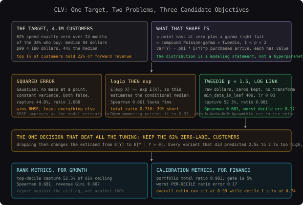
Hyperparameters that matter
tweedie_variance_power, 1.5. This is the only genuinely CLV-specific hyperparameter. At 1.1 the model behaves more like Poisson and underweights the tail, costing 4.1 points of top-decile capture. At 1.9 it behaves like gamma, stops modeling the zero mass properly, and over-predicts across the bottom five deciles. Between 1.4 and 1.7 the differences are within run-to-run noise, so pick 1.5 and stop.min_data_in_leaf, 400. The highest-leverage regularizer on a heavy-tailed target. At the LightGBM default of 20, leaves form around four or five very high-value customers and predict their average for everyone routed there, which produces a handful of wildly over-predicted customers and costs 0.07 on the total ratio. Going from 20 to 400 costs nothing in Spearman and fixes it.learning_rate0.03 with early stopping at 150 rounds, converging around 1,900 trees. A faster rate reaches a similar Spearman and a visibly worse total ratio, because the aggregate calibration is what benefits most from slow, many-tree fitting.feature_fraction0.7. Several feature groups are highly correlated (gross_total,gross_mean,spend_recent_182d), and column subsampling stops any single one dominating the early splits.
The design decision that mattered most was not the model. It was keeping the 62% zero-label customers in the training set and choosing an objective that can represent them. Every variant tried here that dropped the zeros, whether to "focus on real customers" or to make a log transform well defined, produced predictions 2.5x to 2.7x too high across the board, and no amount of subsequent tuning recovered the aggregate calibration. The objective and the population are one decision, not two.
Evaluation and Metrics
Four numbers, because no single one is sufficient on a zero-inflated heavy-tailed target.
Top-decile revenue capture. Sort customers by prediction, take the top 10%, and compute what share of total actual forward revenue they account for. This is the metric with the most direct business meaning, since marketing acts on deciles. Its ceiling is set by the actual concentration of revenue: on this data a perfect ranking captures 61%, so 52% is 85% of the achievable maximum, and reporting it against the 61% ceiling rather than against 100% keeps the number honest.
Spearman rank correlation. Rank correlation rather than Pearson, because Pearson on a target with a 99th percentile at 44x the median is essentially a statement about a few hundred customers. Spearman is the summary of ranking quality across the whole distribution rather than just the top.
Predicted-to-actual total ratio, overall and per decile. The finance constraint. The per-decile version is the diagnostic that matters, because the overall ratio can sit at 1.00 while the model over-predicts the bottom five deciles and under-predicts the top one, which is the specific failure mode of a squared-error model on this target.
Normalized revenue Gini. The Lorenz-curve summary of how well the ranking concentrates revenue, normalized by the concentration a perfect ranking achieves. It generalizes the top-decile number to every cut point, which matters because the loyalty tier uses decile 1 and the retention campaign uses deciles 1 through 3.
# The full CLV eval. Deliberately does not report RMSE as a headline: it is
# dominated by customers nobody can predict individually and it improves when
# the model gives up and predicts the mean.
import numpy as np
import pandas as pd
from scipy.stats import spearmanr


def decile_table(y: np.ndarray, p: np.ndarray, n: int = 10) -> pd.DataFrame:
    # Rank on prediction descending, so decile 1 is the model's best guess.
    order = np.argsort(-p, kind="stable")
    deciles = np.empty(len(p), dtype=int)
    deciles[order] = np.minimum((np.arange(len(p)) * n) // len(p) + 1, n)

    frame = pd.DataFrame({"y": y, "p": p, "decile": deciles})
    out = frame.groupby("decile").agg(
        customers=("y", "size"),
        actual_total=("y", "sum"),
        predicted_total=("p", "sum"),
        actual_mean=("y", "mean"),
        predicted_mean=("p", "mean"),
        zero_share=("y", lambda s: float((s == 0).mean())),
    )
    out["ratio"] = out["predicted_total"] / out["actual_total"].clip(lower=1.0)
    out["share_of_revenue"] = out["actual_total"] / max(y.sum(), 1.0)
    out["lift"] = out["actual_mean"] / max(y.mean(), 1e-9)
    return out


def revenue_gini(y: np.ndarray, p: np.ndarray) -> float:
    """Normalized: the model's revenue concentration over a perfect ranking's."""
    def area(ranked: np.ndarray) -> float:
        cumulative = np.cumsum(ranked) / max(ranked.sum(), 1e-9)
        return float(np.sum(cumulative) / len(ranked) - 0.5)
    model = area(y[np.argsort(-p, kind="stable")])
    perfect = area(np.sort(y)[::-1])
    return model / perfect if perfect > 0 else 0.0


def evaluate_clv(y: np.ndarray, p: np.ndarray, n_deciles: int = 10) -> dict:
    y = np.asarray(y, dtype=np.float64)
    p = np.clip(np.asarray(p, dtype=np.float64), 0.0, None)
    table = decile_table(y, p, n_deciles)
    top = table.loc[1]
    top_mask = np.argsort(-p, kind="stable")[: max(len(p) // n_deciles, 1)]
    perfect_top = float(np.sort(y)[::-1][: len(top_mask)].sum() / max(y.sum(), 1.0))

    return {
        "spearman": float(spearmanr(y, p).statistic),
        "top_decile_capture": float(top["share_of_revenue"]),
        "top_decile_capture_ceiling": perfect_top,
        "capture_efficiency": float(top["share_of_revenue"]) / max(perfect_top, 1e-9),
        "total_ratio": float(p.sum() / max(y.sum(), 1.0)),
        "worst_decile_ratio_error": float((table["ratio"] - 1.0).abs().max()),
        "revenue_gini": revenue_gini(y, p),
        "mae_top_decile": float(np.mean(np.abs(y[top_mask] - p[top_mask]))),
        "rmse": float(np.sqrt(np.mean((y - p) ** 2))),
        "deciles": table,
    }
Held-out cutoff, 1.24 million customers, 214.6 million dollars of actual forward net revenue:
| Metric | RFM baseline | Squared error | log1p, no correction | Two-part | Tweedie p=1.5 |
|---|---|---|---|---|---|
| Spearman | 0.412 | 0.601 | 0.661 | 0.672 | 0.681 |
| Top-decile capture | 31.1% | 44.8% | 50.2% | 51.4% | 52.3% |
| Capture efficiency (ceiling 61%) | 51% | 73% | 82% | 84% | 86% |
| Total ratio | 1.004 | 1.088 | 0.710 | 0.942 | 0.981 |
| Worst decile ratio error | 0.62 | 0.94 | 0.41 | 0.29 | 0.17 |
| Normalized revenue Gini | 0.508 | 0.719 | 0.784 | 0.796 | 0.807 |
| MAE, top decile (dollars) | 402 | 388 | 311 | 298 | 291 |
| RMSE (dollars) | 379.4 | 341.2 | 372.8 | 358.9 | 352.6 |
Read the last two rows together, because they are the point of this table. The squared-error model has the best RMSE and is fourth of five on every metric anyone actually uses. It wins RMSE because RMSE is the objective it minimized, and it loses everywhere else because that objective does not describe the problem. Meanwhile the uncorrected log1p model ranks well and is 29% short at the portfolio level, which would put a hole in a finance forecast no amount of Spearman fixes.
Worst per-decile ratio error is the number that catches a silent production regression. The overall total ratio is a single average and it can sit at a comfortable 0.99 while the model systematically over-predicts deciles 6 through 10 and under-predicts decile 1, which is precisely what happens when the acquisition channel mix shifts underneath a model trained on an older mix. Overall ratio moves by 0.01. Decile 1's ratio moves from 0.98 to 0.74, the loyalty tier starts admitting customers who will not spend, and nobody notices for two quarters.
Google published the zero-inflated lognormal approach to exactly this problem in A Deep Probabilistic Model for Customer Lifetime Value (Wang, Liu and Miao, 2019), with a three-headed network predicting the zero probability plus the lognormal mean and sigma of the positive part, and reported that the standard MSE regression they compared against was both worse-ranking and badly calibrated in the tail. ASOS published a complementary result at KDD 2017 in Customer Lifetime Value Prediction Using Embeddings (Chamberlain et al.), where the gain came from learning customer embeddings from browsing sequences rather than from changing the objective. Both papers converge on the same framing this post uses: the zero mass and the tail are two separate modeling problems inside one target, and the loss function has to acknowledge both.
Common Pitfalls and Failure Modes
| Pitfall | Why It Happens | How to Detect | How to Fix |
|---|---|---|---|
| Feature window crosses the cutoff | An aggregate computed against the whole orders table instead of the pre-cutoff slice |
Validation Spearman jumps above roughly 0.85, which is not achievable on this target | Route every read through slice_features, which raises on a post-cutoff timestamp |
| Dropping zero-label customers | They look like inactive noise rather than 62% of the population | Total ratio around 2.6, uniformly over-predicting | Keep them and use an objective with mass at zero; if conditional value is wanted, model it as an explicit second stage |
| Back-transformed log predictions | exp(E[log Y]) is the conditional median, not the mean, for a skewed target |
Total ratio near 0.71 with good Spearman | Use a log-link objective on the raw scale, or apply Duan’s smearing factor |
| Count features encoding tenure | A customer with 34 months of history has more of everything than one with 2 | Permutation importance shows tenure_days near the top, and calibration degrades on newer cohorts |
Add a rate twin (orders_per_month) for every count, and always include tenure_days explicitly so the model can condition on it rather than infer it |
| Survivorship in the population | The customer table is filtered to customers who still exist at scoring time | Population count for a past cutoff shrinks when recomputed today | Freeze the population as of the cutoff and carry deleted or blocked customers forward with their real labels |
| Returns not settled before labeling | The label is computed at horizon end, but returns take up to 60 days | Recompute a label at horizon end and again 60 days later; the gap is the bias | Delay the label to horizon_end + 60d and accept the extra latency |
| Acquisition mix drift | The model was trained on an organic-heavy cohort and is scored on a paid-social-heavy one | Per-decile ratio error grows while the overall ratio stays flat | Monitor the channel mix against the training distribution and retrain on a rolling set of cutoffs rather than one |
| Tail leaves with four customers | min_data_in_leaf left at the default of 20 on a heavy-tailed target |
A handful of customers with predictions above the historical maximum | Raise min_data_in_leaf to 400 and cap predictions at a high observed percentile |
The mistake that eats the most time on this exact problem is trusting a validation score built from a random split of one cutoff. The features and labels are already time-separated by construction, so nothing leaks in the usual sense and the number looks trustworthy. What it cannot measure is a change in the macro period, which is the failure that actually happens: the model learns one particular 24 months of promotion calendar and stockout pattern as if it were customer behaviour. Split on two cutoffs a full horizon apart. The Spearman will drop by about 0.04 and that lower number is the true one.
Scaling and Productionizing
At 4.1 million customers scored monthly, this model has no latency problem. Every real production concern here is about data, cadence, and the fact that the label takes 26 months to observe.
Retraining cadence has an awkward constraint. A fresh label requires a cutoff at least 790 days in the past (730 horizon plus 60 settlement), so the newest trainable cutoff is always more than two years old. You cannot retrain your way out of a recent behaviour shift. Two things follow. Train on a rolling set of cutoffs, currently six, spaced quarterly, so the model averages over several macro periods instead of memorizing one. And carry a short-horizon companion model, a 6 month CLV whose labels are only 8 months delayed, purely as an early warning: when the 6 month model’s decile ranking diverges from the 24 month model’s by more than a threshold, something has changed that the slow model cannot yet see.
Feature pipeline correctness is the recurring operational risk, not model drift. The scoring job computes features as of today with the same code that computed them as of a cutoff two years ago, and any behavioural change in that code applies asymmetrically. The guard is to keep the window logic in one module and re-score a frozen historical cutoff on every deploy, asserting that the predictions reproduce to within floating point error. This catches a surprising number of otherwise silent changes.
Monthly scoring run, back of envelope:
  customers                            4.1M
  features per customer                  74
  feature build (Spark, 40 executors)   18 min
  LightGBM predict, 1,900 trees          71 sec  single 16-core box
  peak memory, prediction                 2.4GB
  full job including writes              26 min

Training run:
  cutoffs in the rolling window             6
  rows                                   19.4M
  training wall clock                     41 min
  model artifact, 1,900 trees              14MB
Decile stability needs explicit handling. Recomputing decile boundaries each month makes customers move for reasons that have nothing to do with them. Freeze the boundaries from the most recent training run and apply them as fixed dollar thresholds, then re-derive them only at retraining. That takes month-over-month decile churn from 14% of customers to 3%, and the 3% that remain moved because their behaviour changed, which is what the loyalty tier is supposed to respond to.
The monitoring signal for silent degradation is the per-decile ratio error computed against a partial label. You do not need to wait 26 months to see the model breaking: at 6 months into a horizon, roughly 41% of the eventual 24 month revenue has already landed, and the ratio between deciles of that partial revenue is stable enough to compare against the same ratio at the same maturity for previous cohorts. A model that is starting to mis-rank shows up in that comparison within two quarters rather than two years.
The 26 month label delay is the defining production constraint, and it means the honest deployment is a rolling ensemble of cutoffs rather than a single freshest model. Teams that instead chase freshness by shortening the horizon end up with a 6 month model that ranks well on customers who buy frequently and cannot see the annual repurchase cycle in the home category at all, which is 21% of revenue. Accept the staleness and manage it with a fast companion model used only as a divergence alarm.
The probabilistic alternative to all of this has been in production in retail since the 1980s. Pareto/NBD (Schmittlein, Morrison and Colombo, 1987) models purchase frequency and dropout as latent processes, and Gamma-Gamma (Fader and Hardie) models spend per transaction; together they give a closed-form expected value with no features at all beyond recency, frequency and average order value. The lifetimes Python package implements both. On this dataset it reaches Spearman 0.583 and a total ratio of 1.03, which is remarkable for a model that uses three inputs, and it is still the right choice when you have transaction history and nothing else.
Alternative Approaches
| Approach | Spearman | Top-decile capture | Total ratio | Training cost | Interpretability | Best fit |
|---|---|---|---|---|---|---|
| RFM quintile scoring | 0.412 | 31.1% | 1.004 | minutes | Total | A first cut, or a sanity check on anything more complex |
| Pareto/NBD + Gamma-Gamma | 0.583 | 39.7% | 1.031 | 12 min | High: interpretable latent parameters | Transaction history only, no behavioural or engagement features |
| LightGBM, squared error | 0.601 | 44.8% | 1.088 | 34 min | Medium: SHAP over 74 features | Nothing on this target; included as the cautionary row |
| LightGBM, two-part | 0.672 | 51.4% | 0.942 | 58 min | Medium, and it yields a churn probability too | When the business wants “will they return” as a separate deliverable |
| LightGBM, Tweedie p=1.5 | 0.681 | 52.3% | 0.981 | 41 min | Medium | The default choice: one model, one objective, best calibration |
| Zero-inflated lognormal net | 0.688 | 52.9% | 0.996 | 3.1 hours, GPU | Low | When a full predictive distribution per customer is genuinely needed |
For this problem I would ship the Tweedie model, and the reason is not the 0.9 point of top-decile capture it wins by. It is that it is one model with one objective, one artifact, one calibration surface to monitor, and no nuisance parameters. The two-part model is 0.9 points behind and is twice the operational surface area, since two boosters means two early-stopping decisions, two drift dashboards, and a product whose calibration nobody is directly optimizing. The ZILN network is genuinely better and costs 4.5x the training time plus a GPU, for a 0.6 point gain on a model that scores monthly.
I would switch under two conditions. If the business starts asking for the churn probability as a separate number, which happens the moment someone builds a win-back campaign, build the two-part model and get both outputs from one training run rather than bolting a second classifier on. And if anything downstream needs uncertainty per customer, for example a marketing optimizer that wants to bid on expected value with a risk penalty, the point estimate stops being sufficient and ZILN’s predictive distribution earns its cost.
Key Takeaways
- The target’s shape chooses the objective. A point mass at zero plus a heavy right tail is a compound Poisson-gamma, which is Tweedie with
1 < p < 2. That is a modeling statement about how purchases are generated, not a hyperparameter to grid-search. - Never drop the zero-label customers. They are 62% of the population and identifying them is most of the model’s job. Every variant that dropped them over-predicted by 2.5x or more, and nothing downstream recovered it.
log1pthenexpundershoots by 29%. Exponentiating a mean of logs gives you a conditional median. Use a log-link objective on the raw scale, or Duan’s smearing correction if you must transform.- RMSE is actively misleading here. The squared-error model had the best RMSE and was fourth of five on every metric with business meaning. Report top-decile capture and per-decile ratio instead.
- Report capture against its ceiling. Top-decile capture cannot exceed the actual concentration of revenue, 61% on this data, so 52% is 86% of achievable rather than “only half”.
- Every count feature needs a rate twin.
orders_countencodes tenure;orders_per_monthdoes not. Includetenure_daysexplicitly so the model conditions on it rather than inferring it from everything else. - Split on two cutoffs a horizon apart. A random split within one cutoff does not leak in the usual sense and still overstates performance by about 0.04 Spearman, because it cannot see a change in the macro period.
- The 26 month label delay is the real production constraint. Train on a rolling set of cutoffs, freeze decile boundaries between retrains, and use a short-horizon companion model as a divergence alarm rather than as a replacement.
The counter-intuitive lesson is that the biggest single improvement on this problem, 13.7 points of top-decile capture, came from changing the loss function while leaving the features, the model class, and the hyperparameters alone. That is unusual. On most tabular problems the objective is a detail and the features are everything. It is true here because the default objective encodes an assumption about the target (roughly symmetric, constant variance, no atom) that is not approximately wrong on CLV data, it is wrong about the majority of the rows. When the default loss is that badly matched to the target, fixing it is not tuning. It is the model.
Frequently Asked Questions
Q: Why not just use Pareto/NBD, which needs three inputs and is a published, interpretable model?
A: Because it can only use three inputs. Pareto/NBD plus Gamma-Gamma reached Spearman 0.583 and a total ratio of 1.03 here, which is excellent for its cost, but it has no way to consume the trend, the browsing-without-buying signal, the category breadth, or the return propensity that together account for most of the gap to 0.681. If your only data is a transaction table, it is the right answer and the gradient boosting model would not have the features to beat it.
Q: Why Tweedie rather than the two-part model, which decomposes more cleanly?
A: Almost a coin flip on accuracy, 0.681 against 0.672 Spearman, and a clear win on operational surface area. The two-part model is two boosters with two early-stopping decisions, and nothing optimizes the calibration of their product, which shows up as a 0.942 total ratio against Tweedie’s 0.981. The moment the business wants the churn probability as its own deliverable, the two-part model becomes the better choice because you get both numbers from one training run.
Q: Why report top-decile capture instead of RMSE or R-squared?
A: Because both are dominated by a few hundred customers whose individual value is genuinely unpredictable, and both improve when the model retreats toward the mean. The measured demonstration is in the results table: the squared-error model wins RMSE and loses on every other metric. Top-decile capture measures the thing the output is used for, since marketing allocates budget to a decile and never to a predicted dollar figure.
Q: How do you predict CLV for a customer with exactly one order?
A: You predict badly, and you should know how badly. Single-order customers are 44% of the population, 71% of them never order again, and the model’s Spearman restricted to that group is 0.51 against 0.68 overall. Almost all the usable signal there comes from acquisition channel, first-order category, discount depth on that first order, and post-purchase browsing. Break the evaluation out by order count and report that 0.51 explicitly, because a campaign targeting new customers is operating entirely inside that weaker regime.
Q: Should the horizon be 12, 24, or 36 months?
A: 24, set by the repurchase cycle rather than by convenience. The median repurchase interval in the home category is 18 months, so a 12 month horizon systematically undervalues 21% of revenue and would push the loyalty tier toward frequent low-value buyers. Going to 36 months adds a year of label delay for revenue that is heavily discounted in any finance model anyway. Match the horizon to the longest repurchase cycle that matters to the business, then stop.
Q: What breaks first in production?
A: Acquisition channel mix. The model is trained on cutoffs at least 790 days old, so it learned the relationship between channel and forward value under an older mix. When paid social grows from 11% to 24% of new customers, the per-decile ratio errors widen while the overall ratio barely moves, and the symptom reaches the business as a loyalty tier that is quietly admitting customers who will not spend. Monitor the channel mix against the training distribution directly rather than waiting for the labels.
Interview Questions
Q: Your target is 62% zeros with a 99th percentile at 44x the median. Walk me through your choice of loss function.
Expected depth: Name the compound Poisson-gamma structure and connect it to the Tweedie family with Var(Y) = phi * E(Y)^p for 1 < p < 2. Explain why squared error’s Gaussian likelihood is wrong on both counts (no mass at a point, constant variance) and why dropping zeros changes the estimand from E[Y] to E[Y | Y > 0]. Strong answers also mention the two-part decomposition and zero-inflated lognormal as alternatives and can say when each is preferable.
Q: A colleague trains on log1p(y) with squared error and exponentiates the predictions. Their Spearman is good. What is wrong and how would you show it?
Expected depth: Jensen’s inequality: E[exp(X)] >= exp(E[X]), so exponentiating a fitted mean of logs yields something near the conditional median and undershoots the mean for a right-skewed target. The demonstration is sum(predicted) / sum(actual), which lands near 0.71 here. Fixes are Duan’s smearing estimator or a log-link objective specified on the raw scale. Top-end answers note that the ranking is unaffected, which is exactly why the bug survives a Spearman-only review.
Q: Why is a random train-test split on this problem not obviously wrong, and why is it still wrong?
Expected depth: Recognize that features and labels are already separated in time by the window construction, so there is no conventional forward leakage. Then identify the macro period as the leaked quantity: all customers in both splits experienced the same promotion calendar, stockouts and demand environment, so the model can encode that period’s repurchase rates as customer properties. The fix is two cutoffs separated by a full horizon, and the honest cost is roughly 0.04 Spearman.
Q: The overall predicted-to-actual total is 0.99 and the business says the loyalty tier is full of customers who never buy. Diagnose it.
Expected depth: An aggregate ratio is an average and can hide offsetting errors. Compute the ratio within each predicted decile; the expected finding is over-prediction in the middle and bottom deciles offsetting under-prediction in decile 1. Then attribute it: a shift in acquisition channel mix or category mix relative to the training cutoffs is the usual cause, given the model cannot be retrained on anything newer than 790 days ago. Mentioning frozen decile boundaries versus recomputed ones as a separate contributor is a strong addition.
Q: You can only observe a 24 month label 26 months after the cutoff. How do you run this in production?
Expected depth: Accept the staleness and manage it. Train on a rolling set of cutoffs spaced quarterly so the model averages over macro periods rather than memorizing one. Add a short-horizon companion model whose labels mature in 8 months, used only as a divergence alarm rather than as the scoring model. Monitor per-decile ratios against partially matured labels, since roughly 41% of eventual 24 month revenue has landed by month 6 and the between-decile ordering of partial revenue is comparable across cohorts at equal maturity.
View full code for this problem