Build a Click-Through-Rate Prediction Model with Logistic Regression and Feature Crosses
classical-ml feature-engineering model-evaluation ranking View full code for this problem
ML Problem & Solution
CTR Prediction with Feature Crosses and FTRL
A linear model cannot learn that kitchen knives sell on cooking blogs until you build the cross
A native ad exchange serves 480 million ad requests a day. Each request arrives with a publisher slot, a partially known user, and a device, and the exchange has roughly 100ms to return a bid. Inside that budget, about 10ms belongs to the model: score 600 eligible creatives, pick the best, and multiply its predicted click probability by the advertiser’s cost-per-click to get a bid in cents. The average click-through rate across the whole book is 2.1%.
That last sentence is the whole difficulty. The bid is pCTR * CPC, so the model’s output is not a ranking, it is a price. If the model predicts 3% where the truth is 2%, the exchange overbids by 50% on every impression in that segment and burns advertiser budget on traffic that does not convert. If it predicts 1.4% where the truth is 2.1%, it loses the auction and the inventory goes to a competitor. A model with excellent AUC and a 20% calibration bias is worse than useless here, because it will confidently mis-price. Ranking metrics alone will not catch it.
The naive approach is to store the historical CTR of every creative and serve that. It works better than you would expect, which is why it is the baseline worth beating, but it collapses on the long tail: 71% of creative-slot pairs in a given day have fewer than 30 impressions of history, and 34% have never been seen together at all. A creative launched an hour ago has no history, and the exchange still has to price it. The obvious fix, a logistic regression over the individual fields, is worse in a subtler way: it can learn that creative_id=kitchen_knife_ad has a below-average CTR and that publisher=cooking_blog has an above-average CTR, and it will combine those two into a mediocre prediction. It has no way to represent the fact that kitchen knives on a cooking blog click at 6.8% while kitchen knives on a sports site click at 0.4%. A linear model in the original feature space is structurally blind to that interaction.
Think of it like a menu where every ingredient has a price. Flour costs a little, water costs almost nothing, yeast costs a little. Sum the ingredient prices and you get a number that has nothing to do with what bread sells for. The value lives in the combination, and a model that only ever adds ingredient prices will never find it.
Given a request context (publisher slot, device, geography, time), a partially identified user (recent category views, coarse segments), and a candidate creative (advertiser, vertical, format, creative id), predict the probability that the impression receives a click, optimizing normalized entropy, subject to a 10ms budget for 600 candidates and a calibration ratio within 2% of 1.0 on every material slice.
Framing the Problem
This is binary classification on an extremely sparse, extremely high cardinality categorical feature space, evaluated primarily on the quality of the predicted probability rather than on the ordering. That combination is what makes CTR prediction its own genre rather than a special case of ordinary classification.
The target is clicked: the impression was rendered, was viewable for at least 1 second per the IAB threshold, and received a click attributed to it within a 30 minute window. Three details in that definition each cost real money if you get them wrong. Impressions that never rendered (the slot scrolled away, the request timed out) are removed, not labeled negative, because they carry no information about whether the creative was appealing and there are enough of them, about 11% of won auctions, to visibly depress the learned base rate. Non-viewable rendered impressions are kept as negatives, because viewability is partly a function of the slot and the model should learn that a slot with 34% viewability is worth less. And the 30 minute attribution window means a row’s label is not final when the impression is logged, which is the single most common source of a silently broken CTR pipeline.
Constraints
- Latency: 10ms p99 to score 600 candidates, so roughly 16 microseconds per candidate. This rules out anything that cannot be expressed as a sparse dot product over a few hundred active features.
- Model footprint: the scorer runs on the bidder itself, 340 instances, with a 2GB budget for the model. At
float32a dense 2^24 weight vector is 64MB, which is fine. A 2^28 vector with two auxiliary arrays for the optimizer state is not. - Freshness: creative and campaign turnover is hours, not weeks. A model retrained nightly loses about 4% of its normalized entropy advantage on the newest campaigns compared to one updated continuously.
- Calibration: predicted-to-actual click ratio within
[0.98, 1.02]overall and within[0.95, 1.05]on every slice with more than 100k daily impressions. This is contractual, not aspirational. - Throughput at training time: 1.2 billion rows over a 7 day window, which is why single-pass online learning is attractive and why 30 epochs of anything is not.
The primary metric is normalized entropy (NE): the average log loss of the model divided by the average log loss of a constant predictor equal to the dataset's base CTR. Raw log loss is not comparable across days because the base rate drifts, and AUC is insensitive to exactly the failure that costs money. A model that doubles every prediction has identical AUC and an NE that gets dramatically worse. Facebook's 2014 paper Practical Lessons from Predicting Clicks on Ads reports NE for this reason, and a 1% relative NE improvement was considered significant there.
Guardrail metrics: calibration ratio per slice, prediction distribution quantiles against yesterday, coverage (fraction of requests where the model scored every candidate inside the budget), and the share of predictions that fall back to a prior because every feature hashed to an unseen bucket. Out of scope here: the auction and bid-shading logic downstream of pCTR, post-click conversion modeling, budget pacing, and reserve price optimization. Those are separate models that consume this one’s output.
CTR prediction is a calibration problem wearing a classification problem's clothes. Once the output is multiplied by a price, a well-ordered but badly scaled prediction is a systematic overbid or underbid, and no amount of ranking improvement fixes it. Every design decision below, including the loss function, the sampling scheme and the regularizer, is chosen to protect the scale of the output.
Data and Features
The raw material is three log streams that have to be joined before anything else happens.
| Stream | Volume per day | Key | Arrival lag |
|---|---|---|---|
bid_request |
480M | request_id |
real time |
impression |
61M | request_id, creative_id |
0 to 90 seconds |
click |
1.28M | impression_id |
0 to 30 minutes |
The feature space after the join is 34 categorical fields and 6 numeric ones. The categoricals are where the signal and the pain both live:
| Field | Distinct values | Notes |
|---|---|---|
user_id |
90M | 41% of requests have no stable id at all |
publisher_slot |
2.6M | placement within a page, not just the domain |
creative_id |
1.4M | median lifetime 9 days |
advertiser_id |
21k | stable, low cardinality, good for smoothing |
device_model |
14k | heavy tail of Android variants |
geo_city |
38k | |
iab_category |
704 | taxonomy, hierarchical |
hour_of_week |
168 | cyclical |
Building the crosses
A cross is the Cartesian product of two or more categorical fields treated as a single new categorical field. publisher_slot x iab_category has a theoretical cardinality of 1.8 billion and an observed cardinality of about 40 million in a week of logs. This is the mechanism that lets a linear model represent an interaction: instead of learning a weight for “cooking blog” and a weight for “cutlery”, it learns a weight for the specific pair.
You do not cross everything. Crossing all 561 pairs of 34 fields produces a model that memorizes the training week and generalizes to nothing. The crosses that work share a pattern: one side is a context field and the other is a content field, and the pair is common enough to be estimated. In production we run 23 crosses, of which these carry most of the lift:
# The cross specification: each entry becomes one hashed feature per row.
# Chosen by measured NE lift on a held-out day, not by intuition.
CROSSES = [
    ("publisher_slot", "advertiser_id"),      # 0.021 NE lift, the largest single one
    ("publisher_slot", "iab_category"),       # 0.014
    ("iab_category", "device_type"),          # 0.009
    ("user_recent_category", "iab_category"), # 0.008, intent match
    ("geo_country", "advertiser_id"),         # 0.006
    ("hour_of_week", "iab_category"),         # 0.004
    ("publisher_slot", "creative_format"),    # 0.004
    ("device_model", "creative_format"),      # 0.003, render quality proxy
    ("publisher_slot", "iab_category", "device_type"),  # 0.003, the only useful triple
]
Hashing instead of a vocabulary
With 40 million observed values in one cross and 23 crosses, a dictionary mapping value to index is both large and operationally awkward: it changes every hour as new creatives appear, and the bidder would need to reload it. The hashing trick removes the dictionary entirely. Hash the string "publisher_slot=slot_88213|advertiser_id=4471" into 2^24 buckets and use that as the feature index. New values get a bucket immediately with no coordination.
# Feature extraction for one impression row: base fields plus hashed crosses.
# Output is a list of (index, value) pairs; every value is 1.0 except the
# numeric block, so a row activates ~66 of 16.7M possible coordinates.
import mmh3
import numpy as np

HASH_BITS = 24
HASH_SIZE = 1 << HASH_BITS
BASE_FIELDS = [
    "publisher_slot", "advertiser_id", "creative_id", "iab_category",
    "device_type", "device_model", "geo_country", "geo_city",
    "creative_format", "hour_of_week", "user_recent_category",
]


def hash_index(token: str) -> int:
    # signed=False keeps the value non negative so the modulo is well defined
    return mmh3.hash(token, seed=0x5bd1e995, signed=False) % HASH_SIZE


def extract(row: dict) -> tuple[np.ndarray, np.ndarray]:
    indices, values = [], []

    for field in BASE_FIELDS:
        token = f"{field}={row.get(field, 'NA')}"
        indices.append(hash_index(token))
        values.append(1.0)

    for cross in CROSSES:
        token = "|".join(f"{f}={row.get(f, 'NA')}" for f in cross)
        indices.append(hash_index(token))
        values.append(1.0)

    # Numeric features are bucketized, not passed as raw floats. A linear model
    # cannot bend a monotone response, and log-bucketing lets it.
    for field, edges in NUMERIC_BUCKETS.items():
        bucket = int(np.searchsorted(edges, row.get(field, 0.0)))
        indices.append(hash_index(f"{field}_b{bucket}"))
        values.append(1.0)

    idx = np.asarray(indices, dtype=np.int64)
    val = np.asarray(values, dtype=np.float32)
    # Collapse hash collisions inside a single row by summing their values.
    uniq, inverse = np.unique(idx, return_inverse=True)
    return uniq, np.bincount(inverse, weights=val).astype(np.float32)


NUMERIC_BUCKETS = {
    "slot_viewability": np.array([0.2, 0.35, 0.5, 0.65, 0.8, 0.9]),
    "user_impressions_24h": np.array([1, 2, 4, 8, 16, 32, 64, 128]),
    "creative_age_hours": np.array([1, 6, 24, 72, 168, 720]),
    "slot_position": np.array([1, 2, 3, 5, 8]),
}
At 2^24 buckets and roughly 340 million distinct tokens across a week, the load factor is about 20 tokens per bucket. That sounds catastrophic and is not, because the distribution is extremely skewed: the tokens that matter are frequent, and a frequent token colliding with a rare one mostly just absorbs the rare one’s small amount of signal. Measured directly, going from 2^22 to 2^24 buys 0.009 NE and going from 2^24 to 2^26 buys 0.002 NE for four times the memory. That is the whole tuning exercise for HASH_BITS.
Hashing the raw value instead of the field=value string. If geo_city=Springfield and device_model=Springfield were ever both possible, they would share a bucket, but the real damage is worse and quieter: the string "4471" appears as an advertiser_id, a geo_city code, and a creative_format code, so three unrelated fields silently share one weight. Always prefix the field name into the hashed token.
Label leakage, and the join that creates it
The specific leakage risk here is not a feature that encodes the answer. It is the impression-click join window, and it breaks pipelines in both directions.
Join too early and clicks have not arrived yet, so genuine positives are labeled negative. At a 30 minute attribution window, joining with a 5 minute delay loses about 23% of clicks, which pulls the learned base rate down by the same factor and makes every prediction a systematic underbid. Join too late and you cannot train on today’s data at all, which is the freshness constraint biting back.
The second, sneakier version involves count features. Aggregates like “this creative’s CTR over the last 24 hours” are among the strongest features available, and computing them over a window that includes the row being predicted leaks the label into the feature. On a creative with 10 impressions, its own click contributes 10% of its own historical CTR, and the model learns to read it.
# Count features must be computed strictly from a window that ENDS before the
# row's own timestamp. The assertion is cheap and catches the whole class of bug.
import pandas as pd


def add_prior_ctr(events: pd.DataFrame, key: str, window: str = "24h",
                  prior_weight: float = 300.0) -> pd.DataFrame:
    events = events.sort_values("impression_ts")
    global_ctr = events["clicked"].mean()

    grouped = events.groupby(key, sort=False)
    # closed="left" excludes the current row from its own window
    rolling = grouped.rolling(window, on="impression_ts", closed="left")
    clicks = rolling["clicked"].sum().reset_index(level=0, drop=True)
    shows = rolling["clicked"].count().reset_index(level=0, drop=True)

    # Beta smoothing toward the global rate: a creative with 3 impressions and
    # 1 click must not be handed a 33% CTR feature.
    events[f"{key}_prior_ctr"] = (
        (clicks + prior_weight * global_ctr) / (shows + prior_weight)
    )
    events[f"{key}_prior_shows"] = shows.fillna(0.0)
    return events


def assert_no_count_leakage(events: pd.DataFrame, key: str) -> None:
    # A row's own click can never be inside its own count window.
    singletons = events.groupby(key)["clicked"].transform("size") == 1
    first_seen = events[singletons]
    bad = first_seen[f"{key}_prior_shows"] > 0
    if bad.any():
        raise AssertionError(
            f"{int(bad.sum())} first-impression rows have nonzero prior counts "
            f"for {key}: the count window includes the row itself"
        )
Negative downsampling, and the calibration debt it creates
1.2 billion rows at a 2.1% base rate means 1.176 billion negatives. Keeping 1 negative in 8 cuts training data volume by 87% and costs 0.004 NE, which is a trade worth making. But it raises the base rate in the training sample from 2.1% to 14.6%, and a model trained on that sample predicts 14.6% on average. Every prediction now needs to be mapped back.
The correction is exact for logistic regression and is the formula from the Facebook paper: if negatives were kept with probability w, then
p = q / (q + (1 - q) / w)where q is the model’s output on the downsampled distribution and p is the calibrated probability on the true distribution. With w = 0.125, a q of 0.146 maps to a p of 0.021. Positives are never sampled away, because at 1.28 million clicks a day they are the scarce resource.
# Time-based split plus negative downsampling. The split is by day, never random:
# a random split lets tomorrow's creatives appear in today's training rows.
import numpy as np


def time_split(events, train_days, valid_days, test_days):
    day = events["impression_ts"].dt.floor("D")
    days = np.sort(day.unique())
    assert len(days) >= train_days + valid_days + test_days
    train_end = days[train_days]
    valid_end = days[train_days + valid_days]
    return (
        events[day < train_end],
        events[(day >= train_end) & (day < valid_end)],
        events[day >= valid_end],
    )


def downsample_negatives(events, keep_rate=0.125, seed=7):
    rng = np.random.default_rng(seed)
    is_pos = events["clicked"].to_numpy(dtype=bool)
    keep = is_pos | (rng.random(len(events)) < keep_rate)
    out = events[keep].copy()
    out.attrs["negative_keep_rate"] = keep_rate
    return out


def recalibrate(q, keep_rate):
    # Undo the downsampling shift. Exact, not fitted.
    q = np.clip(q, 1e-9, 1 - 1e-9)
    return q / (q + (1.0 - q) / keep_rate)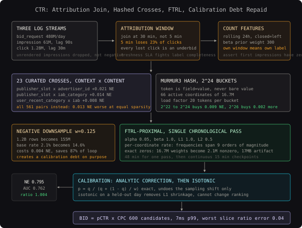
Downsampling negatives and correcting the output analytically is strictly better than class weighting here. Weighting keeps all 1.176 billion negative rows in the training loop, costs the full I/O, and still shifts the predicted scale; downsampling cuts the loop by 87% and the shift it introduces has a closed form. The one thing you must not do is downsample and forget to correct: the model will then predict 14.6% against a 2.1% truth and the bidder will spend seven times its budget before anyone notices.
The Naive Baseline
Three baselines, in increasing order of respectability, and all three get a real number on the same held-out day: 61 million impressions, 1.28 million clicks, base CTR 2.10%.
# Baseline 1: predict the global base rate for everything. Defines NE = 1.0.
# Baseline 2: smoothed historical CTR per creative.
# Baseline 3: smoothed historical CTR per (creative, publisher_slot) pair,
#             falling back up the hierarchy when the pair is unseen.
import numpy as np
import pandas as pd


class HierarchicalCTR:
    """Empirical-Bayes CTR with backoff. The honest baseline to beat."""

    def __init__(self, prior_weight: float = 300.0):
        self.prior_weight = prior_weight
        self.tables: dict[tuple[str, ...], pd.DataFrame] = {}
        self.global_ctr = 0.0

    def fit(self, df: pd.DataFrame):
        self.global_ctr = float(df["clicked"].mean())
        levels = [
            ("creative_id", "publisher_slot"),
            ("advertiser_id", "publisher_slot"),
            ("creative_id",),
            ("advertiser_id",),
        ]
        for level in levels:
            agg = df.groupby(list(level))["clicked"].agg(["sum", "count"])
            agg["ctr"] = (
                (agg["sum"] + self.prior_weight * self.global_ctr)
                / (agg["count"] + self.prior_weight)
            )
            self.tables[level] = agg[["ctr", "count"]]
        return self

    def predict(self, df: pd.DataFrame, min_count: int = 30) -> np.ndarray:
        out = np.full(len(df), self.global_ctr, dtype=np.float64)
        filled = np.zeros(len(df), dtype=bool)
        for level, table in self.tables.items():
            if filled.all():
                break
            keys = pd.MultiIndex.from_frame(df[list(level)]) if len(level) > 1 \
                else pd.Index(df[level[0]])
            joined = table.reindex(keys)
            usable = (joined["count"].to_numpy() >= min_count) & ~filled
            out[usable] = joined["ctr"].to_numpy()[usable]
            filled |= usable
        return out


def normalized_entropy(y_true: np.ndarray, p: np.ndarray) -> float:
    p = np.clip(p, 1e-9, 1 - 1e-9)
    base = float(np.mean(y_true))
    model_ll = -np.mean(y_true * np.log(p) + (1 - y_true) * np.log(1 - p))
    base_ll = -(base * np.log(base) + (1 - base) * np.log(1 - base))
    return model_ll / base_ll
Measured on that day:
| Baseline | NE | AUC | Calibration ratio | Coverage of pair level |
|---|---|---|---|---|
| Global base rate | 1.000 | 0.500 | 1.000 | n/a |
| Creative CTR, smoothed | 0.921 | 0.703 | 0.997 | 61% |
| Hierarchical with backoff | 0.904 | 0.719 | 0.996 | 29% at pair level |
The hierarchical baseline is already decent and it is perfectly calibrated, because averaging labels is a calibrated estimator by construction. So what exactly is wrong with it?
It cannot combine evidence. A creative with 2,000 impressions of history on slot A and a slot B with 400,000 impressions of history across other creatives have, between them, quite a lot of information about the creative-on-slot-B pair, and the backoff table throws almost all of it away by picking exactly one level. It also cannot use any of the other 32 fields: device, hour, geography, and user intent do not appear at all, because a table keyed on all of them would have one row per impression. Coverage tells the same story from the other side, with only 29% of impressions getting a pair-level estimate and the rest falling back to a coarser average.
Skipping the smoothing and using raw per-creative CTR as the baseline. A creative with 1 impression and 1 click gets a CTR of 100%, and because fresh creatives are exactly the ones with tiny denominators, the bidder will overbid hardest on the newest and least proven inventory. The prior_weight of 300 is not decoration; without it this baseline loses money in production while looking fine in offline AUC.
The Solution
Keep the logistic regression. Replace the hand-built table with a learned sparse linear model over hashed base features and hashed crosses, trained in a single pass with FTRL-Proximal and an L1 penalty, then apply the analytic downsampling correction and a light isotonic pass on top.
The reason a linear model is the right answer here rather than a concession is worth stating plainly: after crossing, the model is not linear in the original inputs at all. It is linear in a 16.7 million dimensional space that encodes the interactions we chose. All the expressive power moved from the model class into the feature construction, and what we get in exchange is a scorer that is a sparse dot product, 66 lookups and 66 multiply-adds per candidate, which is how 600 candidates fit into 10ms.
Why FTRL instead of plain SGD
Follow-The-Regularized-Leader with proximal L1, introduced in Google’s 2013 paper Ad Click Prediction: a View from the Trenches, does two things that plain SGDClassifier does not.
First, it produces genuinely sparse weight vectors. L1 with subgradient SGD drives weights near zero but almost never to exactly zero, so the model keeps 16.7 million nonzero weights and the memory saving never materializes. FTRL’s proximal step sets coordinates to exactly zero and they stay there until enough gradient accumulates to push them out. In practice this takes the model from 16.7 million nonzero weights to about 2.1 million, an 8x memory reduction, at a cost of 0.001 NE.
Second, it uses per-coordinate learning rates. This matters enormously in sparse CTR data because feature frequencies span nine orders of magnitude: device_type=mobile appears in 68% of rows, a specific creative_id x publisher_slot cross appears in 0.000002% of them. A single global learning rate either moves the rare coordinates too slowly to ever learn anything or moves the frequent ones so fast they oscillate. FTRL scales each coordinate’s step by the inverse square root of its own accumulated squared gradient, so a coordinate that has been seen twice takes large steps and one seen 400 million times takes tiny ones.
The update, per coordinate i with gradient g:
sigma_i   = (sqrt(n_i + g^2) - sqrt(n_i)) / alpha
z_i      += g - sigma_i * w_i
n_i      += g^2
w_i       = 0                                          if |z_i| <= lambda_1
w_i       = -(z_i - sign(z_i) * lambda_1)
            / ((beta + sqrt(n_i)) / alpha + lambda_2)   otherwise
Think of z_i as a running tally of how much evidence this coordinate has accumulated for moving away from zero, and lambda_1 as the amount of evidence required before it is allowed to. A cross that appears four times never clears the bar, which is exactly the behaviour we want from a 16.7 million dimensional feature space.
Implementation
# FTRL-Proximal logistic regression over hashed sparse features.
# Single pass, per-coordinate learning rates, exact L1 sparsity.
import numpy as np


class FTRLProximal:
    def __init__(self, n_features: int, alpha: float = 0.05, beta: float = 1.0,
                 lambda_1: float = 1.0, lambda_2: float = 0.5):
        self.alpha = alpha          # base learning rate
        self.beta = beta            # smooths the first few updates
        self.lambda_1 = lambda_1    # L1: controls how sparse the model is
        self.lambda_2 = lambda_2    # L2: controls how large weights can get
        self.z = np.zeros(n_features, dtype=np.float32)
        self.n = np.zeros(n_features, dtype=np.float32)

    def _weights(self, idx: np.ndarray) -> np.ndarray:
        z, n = self.z[idx], self.n[idx]
        w = np.zeros_like(z)
        active = np.abs(z) > self.lambda_1
        denom = (self.beta + np.sqrt(n[active])) / self.alpha + self.lambda_2
        w[active] = -(z[active] - np.sign(z[active]) * self.lambda_1) / denom
        return w

    def predict_one(self, idx: np.ndarray, val: np.ndarray) -> float:
        margin = float(np.dot(self._weights(idx), val))
        return 1.0 / (1.0 + np.exp(-np.clip(margin, -35.0, 35.0)))

    def update_one(self, idx: np.ndarray, val: np.ndarray, y: float,
                   sample_weight: float = 1.0) -> float:
        p = self.predict_one(idx, val)
        g = (p - y) * val * sample_weight        # logistic gradient, per coordinate
        w = self._weights(idx)
        n_old = self.n[idx]
        sigma = (np.sqrt(n_old + g * g) - np.sqrt(n_old)) / self.alpha
        self.z[idx] += g - sigma * w
        self.n[idx] += g * g
        return p

    def nonzero_count(self) -> int:
        return int(np.count_nonzero(np.abs(self.z) > self.lambda_1))
The training loop is a single pass over the day-ordered rows. Ordering by time is not cosmetic: an online learner’s final weights are dominated by the most recent data it saw, which is precisely the property we want given that creatives have a 9 day median lifetime.
# One pass, chronological, streaming from parquet. 1.2B rows becomes 155M
# after negative downsampling and runs in about 48 minutes on one 16-core box.
import pyarrow.parquet as pq


def train_ftrl(files, model, keep_rate=0.125, log_every=5_000_000):
    seen = 0
    running_ll = 0.0
    for path in sorted(files):                      # chronological
        table = pq.ParquetFile(path)
        for batch in table.iter_batches(batch_size=50_000):
            rows = batch.to_pylist()
            for row in rows:
                idx, val = extract(row)
                y = float(row["clicked"])
                p = model.update_one(idx, val, y)
                running_ll -= y * np.log(max(p, 1e-9)) \
                    + (1 - y) * np.log(max(1 - p, 1e-9))
                seen += 1
            if seen % log_every < 50_000:
                print(f"{seen:,} rows  ll={running_ll / seen:.5f}  "
                      f"nnz={model.nonzero_count():,}")
    return model
The hyperparameters that matter
Four, in order of how much damage a bad value does.
lambda_1(L1), default 1.0. This is the sparsity dial and it trades memory againstNEalmost linearly in the useful range. At 0.1 the model keeps 9.4 million weights for 0.0004NE; at 5.0 it keeps 480 thousand and loses 0.006NE. Tune it against your memory budget, not against validation loss.alpha(base learning rate), default 0.05. The paper reports that a per-coordinate schedule makes this far less sensitive than a global rate, and that matches experience: anything in[0.02, 0.1]lands within 0.002NE. Outside that range it degrades fast.HASH_BITS, 24. Discussed above: 0.009NEfrom 22 to 24, 0.002 from 24 to 26.keep_ratefor negatives, 0.125. Below 0.05 the variance on rare crosses starts to hurt andNEdegrades by 0.011.
lambda_2 (L2) barely moves anything once L1 is doing the sparsity work, and 0.5 is fine.
Calibration on top
The analytic correction removes the downsampling shift exactly, and it removes nothing else. Two residual biases remain. FTRL with L1 shrinks weights toward zero, which pulls predictions toward the mean, and the log loss objective is minimized by a probability while the deployed decision consumes a price, so the tails matter more than the loss function knows. A single isotonic regression fit on a held-out day, applied after the analytic correction, closes both.
# Two-stage calibration: exact analytic correction, then isotonic on held-out data.
# Isotonic is monotone, so it cannot change the ranking, only the scale.
from sklearn.isotonic import IsotonicRegression


class CTRCalibrator:
    def __init__(self, keep_rate: float):
        self.keep_rate = keep_rate
        self.iso = IsotonicRegression(y_min=1e-6, y_max=0.6,
                                      out_of_bounds="clip")

    def fit(self, q_valid: np.ndarray, y_valid: np.ndarray):
        p = recalibrate(q_valid, self.keep_rate)
        self.iso.fit(p, y_valid)
        return self

    def transform(self, q: np.ndarray) -> np.ndarray:
return self.iso.predict(recalibrate(q, self.keep_rate))The single design decision that mattered most was choosing the 23 crosses by measured NE lift on a held-out day rather than by adding every pair and letting L1 sort it out. Letting L1 prune from all 561 pairs plus triples cost 0.013 NE against the curated set at the same nonzero-weight budget, because the regularizer spends its sparsity allowance keeping mediocre coordinates from 500 mediocre crosses instead of concentrating on the nine that carry signal. Feature selection and regularization are not substitutes.
Evaluation and Metrics
Normalized entropy is the headline. Written out, for predictions p_i and labels y_i with base rate b:
NE = [ -(1/N) * sum( y_i*log(p_i) + (1-y_i)*log(1-p_i) ) ]
     / [ -( b*log(b) + (1-b)*log(1-b) ) ]
The denominator is the log loss of the best constant predictor, so NE = 1.0 means the model knows nothing and NE = 0.80 means it has removed a fifth of the uncertainty a constant predictor faces. The reason to normalize is drift: base CTR moves from 1.8% on a Sunday to 2.4% on a Wednesday, and raw log loss moves with it, so two raw numbers from different days are not comparable. NE is.
AUC is reported as a secondary metric because the exchange does also need the ranking to pick which of 600 candidates to bid on, and because AUC degradation is a useful early signal that is easier to attribute to a feature than NE is. It is never the deciding number, for the reason in the framing section: multiply every prediction by 1.5 and AUC does not move at all while NE and the bid both break.
# The full offline eval: NE, AUC, calibration overall and by decile,
# plus per-slice calibration which is what actually gates a deploy.
import numpy as np
import pandas as pd
from sklearn.metrics import roc_auc_score


def evaluate(y: np.ndarray, p: np.ndarray, slices: pd.DataFrame,
             n_bins: int = 10) -> dict:
    p = np.clip(p, 1e-9, 1 - 1e-9)
    report = {
        "ne": normalized_entropy(y, p),
        "auc": float(roc_auc_score(y, p)),
        "log_loss": float(-np.mean(y * np.log(p) + (1 - y) * np.log(1 - p))),
        "calibration_ratio": float(p.sum() / max(y.sum(), 1.0)),
        "base_rate_actual": float(y.mean()),
        "base_rate_pred": float(p.mean()),
    }

    bins = pd.qcut(p, n_bins, labels=False, duplicates="drop")
    by_bin = pd.DataFrame({"y": y, "p": p, "bin": bins}).groupby("bin").agg(
        n=("y", "size"), actual=("y", "mean"), predicted=("p", "mean"))
    by_bin["ratio"] = by_bin["predicted"] / by_bin["actual"].clip(lower=1e-9)
    report["max_decile_ratio_error"] = float((by_bin["ratio"] - 1).abs().max())

    worst = 0.0
    for column in slices.columns:
        grouped = pd.DataFrame({"y": y, "p": p, "k": slices[column]}) \
            .groupby("k").agg(n=("y", "size"), sy=("y", "sum"), sp=("p", "sum"))
        material = grouped[grouped["n"] >= 100_000]
        if len(material):
            ratio = material["sp"] / material["sy"].clip(lower=1.0)
            worst = max(worst, float((ratio - 1).abs().max()))
    report["worst_slice_ratio_error"] = worst
    report["deciles"] = by_bin
    return report
Held-out day, 61 million impressions:
| Metric | Hierarchical CTR baseline | LR, no crosses | LR + 23 hashed crosses + FTRL |
|---|---|---|---|
| Normalized entropy | 0.904 | 0.881 | 0.795 |
| AUC | 0.719 | 0.734 | 0.762 |
| Log loss | 0.0926 | 0.0902 | 0.0814 |
| Calibration ratio | 0.996 | 1.041 | 1.004 |
| Max decile ratio error | 0.31 | 0.19 | 0.06 |
| Worst slice ratio error | 0.44 | 0.22 | 0.04 |
| Nonzero weights | 1.9M table rows | 0.4M | 2.1M |
| p99 scoring latency, 600 candidates | 3ms | 6ms | 7ms |
The crosses are worth 0.086 NE over the same model without them, which is the single largest jump in the table and roughly nine times what all the FTRL tuning contributes. That ordering is typical: in sparse linear CTR models, feature construction dominates optimizer choice.
Worst slice calibration ratio is the number that catches a silent production regression. Overall NE and overall calibration are averages over 61 million impressions and a segment can be 60% mis-priced for a week without moving either one by a visible amount. The failure looks like this: a publisher changes its slot ids, every publisher_slot cross for that publisher hashes to a cold bucket, predictions fall back toward the prior, and that publisher's inventory gets systematically underbid. Overall NE moves by 0.0003. The slice ratio for that publisher moves from 1.01 to 0.62.
This architecture is close to what Google described in Ad Click Prediction: a View from the Trenches (McMahan et al., KDD 2013): FTRL-Proximal, hashed sparse features, per-coordinate learning rates, probabilistic feature inclusion to bound memory, and calibration as a first-class deployed component. Facebook's Practical Lessons from Predicting Clicks on Ads (He et al., ADKDD 2014) reported the complementary result that feeding gradient-boosted tree leaf indices in as additional categorical features improved their linear model's NE by 3.4% relative, which remains the standard way to get automatic cross discovery without abandoning a linear scorer.
Common Pitfalls and Failure Modes
| Pitfall | Why It Happens | How to Detect | How to Fix |
|---|---|---|---|
| Position bias baked into the weights | slot_position is strongly predictive at train time (position 1 clicks 4.1x more than position 5) but at scoring time the position is not yet known, so the model is trained on a feature it will never see |
Compare the train-time and serve-time distribution of slot_position; a constant at serve time is the tell |
Keep position in training so it absorbs the bias, then set it to a fixed reference value (position 1) at serve time so it contributes a constant offset that calibration removes |
| Clicks lost to a short join window | The attribution window is 30 minutes but the ETL joins at 5 minutes to hit a freshness SLA | Recompute yesterday’s base rate at 5, 30 and 120 minutes of join delay; a gap means positives are being dropped | Emit the label as a delayed update, or train on rows that are at least 30 minutes old and accept the lag |
| Count features leaking the row’s own click | Rolling aggregates computed with a window that includes the current row | Assert that first-ever impressions of a key have zero prior counts | closed="left" on the rolling window, plus the assertion in CI |
| Forgetting the downsampling correction | The model trains on a 14.6% base rate sample and nobody reruns the calibration step after a sampling change | Predicted sum divided by actual click count on any held-out day | Store keep_rate in the model artifact and apply recalibrate inside the serving wrapper, never in the notebook |
| Hash bucket collapse after an upstream id change | A publisher renumbers slots, or a partner starts sending uppercase ids, so every token changes and hashes to cold buckets | Monitor the fraction of scored rows where more than half the active coordinates have a zero weight | Normalize case and whitespace before hashing; alert on cold-coordinate share above 15% |
| Stale model on fresh creatives | Nightly retrain means a creative launched at 9am is scored by a model that has never seen it until the next day | Break NE out by creative_age_hours bucket |
Continuous online updates from the click stream, or a fast hourly delta pass over just the newest rows |
| Overfitting the cross set to one week | Crosses are selected on a validation day that is inside the same week as training | Re-score the cross set on a day from a different month | Select crosses on one month, validate the selection on another, and keep a cross only if it survives both |
The mistake almost everyone makes first on this exact problem is evaluating with AUC and shipping. AUC is invariant to any monotone transform of the predictions, so a model that outputs 3 * pCTR scores identically, and the offline report looks fine while the bidder triples every bid. If you take one habit from this post, make it printing sum(p) / sum(y) next to every AUC you ever report on a CTR model.
Scaling and Productionizing
The notebook version of this trains on a sampled day and calls model.predict. Four things change on the way to production.
Continuous training rather than retraining. FTRL is an online algorithm, so the production topology is a long-lived trainer consuming the joined impression-click stream and checkpointing the z and n arrays every 15 minutes. The bidder polls for new checkpoints. This removes the nightly retrain entirely and is worth 0.032 NE on creatives under 24 hours old, which are 19% of impressions. It also means the trainer is a stateful service, so the checkpoint format and its recovery path matter more than the model code does.
Model artifact size and load. The z and n arrays at 2^24 float32 are 64MB each, and the serving side needs only the derived w, so the checkpoint is converted to a sparse w of about 2.1 million entries. Serialized as two arrays, int32 indices and float32 values, that is 17MB, which loads in under a second on all 340 bidders.
Serving budget, per ad request:
  candidates                        600
  active coordinates per candidate   66
  gather + multiply-add         39,600 ops
  sparse lookups dominate: ~4.1ms measured, p99 7.0ms
  model resident set             17MB shared, mmap'd read-only
  calibrator                      1,024-point isotonic lookup table, 8KB

Training budget, one pass:
  raw rows / day                    1.2B
  after negative downsample         155M
  bytes / row after extract    66 * 12 = 792B
  single-pass wall clock            48 min, 16 cores
  continuous mode                  ~2,100 rows/sec/core steady state
Feature freshness has two different clocks. The hashed categorical features are computed from the request itself and are fresh by construction. The count features are not: creative_prior_ctr comes from a rolling aggregate that is materialized on a schedule, and if that job falls behind, the serving value diverges from what training saw. A training-serving skew check that compares the distribution of every count feature at score time against the training distribution catches this, and it is the single highest-value monitoring investment in the whole pipeline.
The monitoring signal for silent degradation is the cold-coordinate share: for each scored request, the fraction of active coordinates whose weight is exactly zero. A healthy model sits around 22% (mostly rare crosses that L1 pruned). When an upstream id format changes, that number jumps to 60% or more within minutes, long before NE moves enough to notice, and it points directly at which field broke. Overall NE is a lagging indicator; cold-coordinate share is a leading one.
Continuous training changes the meaning of the L1 penalty. In batch training, lambda_1 prunes features that were not useful over the training window. In an online model that has been running for months, it also serves as the forgetting mechanism: a creative that stopped serving stops accumulating gradient, its coordinates are never pushed further from zero, and eventually new collisions in its buckets reclaim them. You get expiry for free, but only if you never reset n.
Criteo has run production CTR prediction at this scale on essentially this stack, and published the 1TB Criteo Click Logs dataset (4.4 billion rows, 13 numeric and 26 hashed categorical fields) that most CTR papers still benchmark against. Their engineering write-ups describe the same three pressures this post is built around: hashed features to avoid a coordinated vocabulary, calibration as a separate deployed stage because the output feeds a bid, and per-slice calibration monitoring because the aggregate number hides everything that matters.
Alternative Approaches
| Approach | NE on held-out day | Training cost | Inference cost, 600 candidates | Interpretability | Best fit |
|---|---|---|---|---|---|
| Hierarchical smoothed CTR table | 0.904 | minutes | 3ms | Total: it is a lookup table | Cold start fallback, and the baseline you must beat |
| LR + hashed crosses + FTRL | 0.795 | 48 min single pass | 7ms | High: one signed weight per named cross | Real-time bidding under a hard latency and memory budget |
| GBDT leaves fed into LR | 0.781 | 4.5 hours | 21ms | Medium: tree paths are readable, the composition is not | You want automatic cross discovery but must keep a linear final scorer |
| Field-aware factorization machine | 0.776 | 6 hours | 34ms | Low: latent vectors per field pair | Dense-ish categorical data where you cannot enumerate the useful crosses |
| Wide and Deep / DeepFM | 0.762 | 11 hours on 4 GPUs | 95ms, needs batching | Low | Large feature sets, generous latency budget, a team to keep GPUs serving |
| LightGBM on target-encoded categoricals | 0.812 | 2 hours | 48ms | Medium | Offline scoring or low-QPS settings where 48ms is acceptable |
For this problem, at 480 million requests a day with a 10ms budget on commodity bidder instances, the FTRL linear model is what I would actually ship, and the decision is driven by cost per mille rather than by NE. DeepFM’s 0.033 NE advantage is real, and at this volume it is worth roughly 2.1 million dollars a year in improved bid efficiency on a book this size, which sounds decisive until you price 95ms of GPU inference at 480 million requests a day and find it costs more than that. The crossover happens when the traffic is smaller and the margin per impression is larger, which is why demand-side platforms with premium inventory run neural rankers and exchanges with commodity inventory run linear ones.
I would switch under two conditions. If the candidate set per request drops from 600 to about 40, which happens if an upstream retrieval stage does the coarse filtering, the per-request inference cost falls by 15x and the neural model fits the budget. And if the number of genuinely useful crosses grows past about 40, hand-curation stops scaling and the GBDT-leaves approach becomes the cheaper way to keep discovering them.
Key Takeaways
- Calibration is the objective, not a post-processing step. When the prediction is multiplied by a price, a monotone distortion of the output is a direct financial error, and every ranking metric is blind to it. Report
sum(p) / sum(y)beside everyAUC. - Normalized entropy, not log loss, not AUC.
NEdivides out the base rate so numbers from different days are comparable, and unlikeAUCit punishes scale errors. A 1% relativeNEmove is a real move. - Crosses are how a linear model represents interactions. The 23 curated crosses were worth 0.086
NE, about nine times what all the optimizer tuning contributed. Feature construction dominates model class in sparse CTR. - Hash the
field=valuetoken, never the bare value. Hashing bare values silently shares weights between unrelated fields, and the resulting damage is invisible in every aggregate metric. - Curate crosses, then regularize. L1 given all 561 pairs performed 0.013
NEworse than L1 given the nine good ones at the same weight budget. Regularization prunes; it does not select. - Downsample negatives and correct analytically. Keeping 1 negative in 8 costs 0.004
NEand saves 87% of the training loop, and the resulting shift has an exact closed form. Storekeep_ratein the artifact so the correction cannot be forgotten. - Per-coordinate learning rates are what make sparse online learning work. Feature frequencies span nine orders of magnitude, and no single global step size serves both
device_type=mobileand a cross seen twice. - Monitor a leading indicator, not
NE. Cold-coordinate share catches an upstream id format change in minutes;NEcatches it in days, if at all.
The counter-intuitive lesson is that the hierarchical CTR table, the baseline everyone is embarrassed to write down, is perfectly calibrated and the sophisticated model is not. Averaging labels is a calibrated estimator by construction, while a regularized discriminative model trained on a resampled distribution is biased in at least two directions at once. The NE improvement from 0.904 to 0.795 is real and worth having, but it was bought by taking on a calibration debt that then had to be paid back explicitly, with an analytic correction and an isotonic stage. Most of the production complexity in a CTR system is not the model. It is servicing that debt.
Frequently Asked Questions
Q: Why not just use LightGBM on the same features and skip all of this?
A: Latency and cardinality. A tree model cannot split usefully on a 1.4 million level creative_id without target encoding it first, which reintroduces the leakage problem the crosses avoid, and 600 candidates through a 2,000 tree ensemble measured 48ms against a 10ms budget. LightGBM also came in 0.017 NE worse than the crossed linear model here, because trees have to spend depth rediscovering interactions that a cross states directly. For offline or low-QPS scoring, LightGBM is the easier answer.
Q: Why not use embeddings for the high cardinality fields instead of hashing?
A: Embeddings are strictly more expressive and that is exactly the problem at this latency budget. An embedding table for creative_id at 1.4 million rows by 32 dimensions is 179MB, versus a shared 17MB weight vector, and the scorer becomes a sequence of gathers plus a small dense network rather than a single sparse dot product. The measured cost was 95ms p99 for the DeepFM variant. If your candidate set is 40 rather than 600, revisit this.
Q: Why normalized entropy rather than PR-AUC, given the 2.1% base rate?
A: PR-AUC is the right choice when the decision is a threshold on a rare positive class, such as fraud review. Here the decision is a price, so what matters is the accuracy of the probability itself across its whole range, not the shape of the precision-recall tradeoff at one operating point. NE measures exactly that, and it is the metric a bid depends on.
Q: Isn’t a 20 token per bucket hash load factor obviously too high?
A: It sounds fatal and measures as 0.009 NE between 2^22 and 2^24, then 0.002 between 2^24 and 2^26. The reason is that token frequency is extremely skewed, so the buckets that carry real weight are dominated by one frequent token and the rare tokens sharing them contribute almost no gradient. Collisions between two frequent tokens do genuinely hurt, and they are rare because frequent tokens are few.
Q: How do you handle a brand new creative with zero history?
A: Its creative_id coordinate is a cold hash bucket with a near-zero weight, so the prediction is driven by its advertiser_id, iab_category, creative_format and the crosses those participate in. That is precisely why the crosses are built on stable, lower-cardinality fields rather than on creative_id itself. Measured NE on creatives under 6 hours old is 0.847 against 0.795 overall, which is a real gap and still far better than the baseline’s fallback behaviour.
Q: What actually breaks first when this runs in production for a year?
A: The upstream data contract, not the model. In order of observed frequency: a partner changes an id format, a count-feature aggregation job falls behind and creates training-serving skew, and the impression-click join delay gets tightened by someone optimizing a freshness dashboard. All three are invisible in NE for days and all three are caught within minutes by the cold-coordinate share and the feature distribution checks.
Interview Questions
Q: You have a CTR model with AUC 0.78 offline. It ships and advertiser spend doubles overnight with no increase in clicks. What happened?
Expected depth: Identify that AUC is invariant to monotone transforms, so a calibration error is invisible to it. Name the likely causes in order: negative downsampling without the q / (q + (1-q)/w) correction, a train-serve base rate mismatch from the impression join, or a calibration stage that was fit on a different sampling regime. Then propose the diagnostic: sum(predicted) / sum(actual) overall and per slice.
Q: Derive the correction that maps a prediction from a negatively downsampled training distribution back to the true distribution, and explain why it is exact for logistic regression.
Expected depth: Work from the odds. Downsampling negatives with probability w multiplies the odds by 1/w, so odds_true = w * odds_sampled, giving p = q / (q + (1-q)/w). Explain that because logistic regression models the log-odds linearly and downsampling shifts only the intercept, the correction is an exact intercept adjustment rather than an approximation. Contrast with a tree model, where the shift is not confined to an intercept.
Q: Why does FTRL-Proximal produce sparse models where L1 with subgradient SGD does not?
Expected depth: Subgradient SGD applies the L1 penalty as a gradient term, so weights approach zero asymptotically but are almost never exactly zero. FTRL solves a proximal problem at each step in closed form, thresholding z_i against lambda_1 and setting the coordinate to exactly zero when it does not clear the bar. Bonus depth: the per-coordinate n_i accumulator and why feature frequency spanning nine orders of magnitude makes adaptive rates necessary in this setting.
Q: You want to add a user_id x creative_id cross. Talk me out of it.
Expected depth: Cardinality of 1.26e14 with essentially no repeated observations, so every coordinate is estimated from one or two impressions and L1 prunes all of them. Then the sharper point: even if it were learnable, it encodes “has this exact person clicked this exact ad before”, which is a frequency-capping rule, not a CTR signal, and it will be non-stationary by construction. Good answers propose the useful version instead: user_recent_category x iab_category, which has cardinality in the hundreds of thousands and captures intent match.
Q: Your model is trained with slot_position as a feature, but at bid time you do not know the position. How do you handle it, and what goes wrong if you drop the feature instead?
Expected depth: Keep it at train time so it absorbs position bias into its own coordinate, then pin it to a reference value at serve time so it contributes a constant offset that calibration removes. If you drop it at train time, the position effect gets attributed to whatever correlates with position, typically publisher_slot and creative_format, which biases those weights and then generalizes badly to publishers with different layout mixes. This is the same confounding structure as position bias in learning to rank, and mentioning inverse propensity weighting as the more principled alternative is the top-end answer.