Build a Multi-Class Product Categorization Classifier with Naive Bayes and TF-IDF
classical-ml nlp feature-engineering model-evaluation View full code for this problem
ML Problem & Solution
Product Categorization with Naive Bayes and TF-IDF
1,200 classes, 9 words of input, and a 50ms budget. Accuracy will lie to you about all three.
A marketplace lets sellers list anything, and every listing has to land in exactly one of 1,200 leaf categories in the browse taxonomy. Category drives search filters, shipping rules, commission rates, and tax treatment, so a misfiled listing is not a cosmetic problem: a phone case filed under “Cell Phones” instead of “Cell Phone Accessories” shows up when a buyer filters for phones under 300 dollars, and the seller pays the wrong commission rate.
Sellers pick the category themselves during listing creation, and they get it wrong roughly 12% of the time. Some of that is honest confusion between sibling categories. Some is deliberate, because the highest-traffic category is not always the correct one. The listing form has the category dropdown, so the current system is already an ML problem in disguise: the seller’s choice is a noisy label, and the platform needs a model that can disagree with it.
What the model gets is thin. A seller-written title averaging 9 tokens, a description that is empty on 31% of listings, and a brand field that is free text and empty on 44%. Titles look like Apple iPhone 13 Pro Max Case Clear Shockproof TPU Bumper 6.7" or Vtg 90s Nike Windbreaker Mens L Teal Colorblock. They are keyword-stuffed, abbreviation-heavy, inconsistently cased, and full of model numbers that carry more signal than any English word in the string.
The naive approach is a keyword rule table, and it fails in a specific and instructive way. Rules get you to about 45% accuracy on the top 50 categories and essentially nothing on the tail, because the rule table is maintained by hand and nobody maintains 1,200 of them. Worse, rules collide: case appears in “Cell Phone Accessories”, “Camera Cases”, “Musical Instrument Cases”, and “Wine Cases”, and the priority order that resolves those collisions becomes an unreviewable 4,000-line file. The second naive approach, an off-the-shelf multilingual embedding model plus nearest neighbor, misses the point in the other direction: it captures semantic similarity beautifully and treats iPhone 13 and iPhone 14 as near-identical, which is exactly the distinction the taxonomy cares about.
Think of it as sorting mail in a building with 1,200 mailboxes where each envelope has a nine-word address written by a different person, and 300 of those mailboxes get one envelope a month. The hard part is not the busy mailboxes. It is that a metric measured over envelopes tells you almost nothing about the 300 quiet ones.
Given a listing title, optional description, and optional brand string, predict the single correct leaf category out of 1,200, optimizing macro-F1 so tail categories count, under a 50ms p99 latency budget at listing-submission time.
Framing the Problem
This is single-label multi-class classification over 1,200 mutually exclusive classes, with a taxonomy structure (6 top-level departments, roughly 90 mid-level nodes, 1,200 leaves) that the flat formulation ignores and the evaluation should not.
The target is the leaf category ID. Ground truth is the seller’s selection, corrected by two sources: the 4.1% of listings that were manually recategorized by the trust and safety team, and the 1.8% that were recategorized after a buyer report. Those corrections are the cleanest labels in the dataset and they are also not randomly sampled, since they concentrate on listings that got traffic. That biases the correction set toward popular categories, which matters for how much we trust evaluation on the tail.
The class distribution is brutal and drives every subsequent decision:
| Segment | Categories | Share of listings | Median listings per category |
|---|---|---|---|
| Head | 50 | 61.2% | 24,100 |
| Torso | 310 | 31.7% | 1,840 |
| Tail | 840 | 7.1% | 64 |
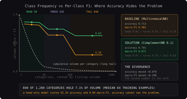
840 of 1,200 categories hold 7.1% of the volume between them, and the median tail category has 64 training examples.
Constraints:
- Latency: 50ms p99, inline in the listing-submission request. The model is one of four calls in that handler.
- Training time matters. The taxonomy changes monthly (categories get split, merged, deprecated), so a full retrain has to fit comfortably inside a CI job, not a GPU reservation.
- No GPU at serving time. The model runs on the same commodity application pods as the rest of the listing service.
- Partial automation is acceptable and expected. The model does not have to decide every listing. It can auto-accept high-confidence predictions, suggest for low-confidence ones, and route the genuinely ambiguous to a human queue that has capacity for about 3% of daily volume.
- Cold start on new categories. A category created this month has zero training examples and still needs to be reachable.
Success metric: macro-F1 across all 1,200 classes, which weights the 64-example tail category exactly as heavily as the 24,100-example head category.
Guardrail metrics: weighted-F1 must not regress (that is the buyer-visible quality), top-3 accuracy must stay above 0.90 (that drives the suggestion UI), and the share of volume routed to human review must stay under 3%.
Accuracy is actively misleading here. A model that predicts only the top 50 categories and refuses to ever emit a tail label scores 61.2% accuracy and a macro-F1 of 0.04. Every improvement that moves accuracy without moving macro-F1 is an improvement that made the head better and the tail worse.
Out of scope: multi-label listings (a bundle that legitimately spans categories), image signals from listing photos, cross-lingual listings, and the taxonomy design itself. This post is the text-only, single-label classifier.
The 1,200-way flat formulation is a modeling simplification, not a description of the problem. The taxonomy is a tree, sibling confusions cost far less than cross-department confusions, and both the fallback strategy and the evaluation should use that structure even when the classifier itself does not.
Data and Features
2.8M listings with a label, spanning 18 months. Three text fields, all seller-written:
| Field | Missing | Avg tokens | Notes |
|---|---|---|---|
title |
0% | 9.2 | Keyword-stuffed, abbreviation-heavy, model numbers throughout |
description |
31% | 47.0 | When present, often boilerplate shipping and returns text |
brand |
44% | 1.4 | Free text, so Nike, NIKE, and nike inc are three distinct strings |
Why two vectorizers instead of one
The signal in a product title splits into two kinds of token, and one vectorizer cannot capture both.
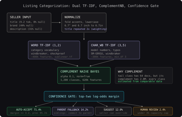
Word n-grams capture the category vocabulary: windbreaker, shockproof, bumper, colorblock. Unigrams plus bigrams, because phone case and case phone should not be distinguishable but phone case and camera case very much should.
Character n-grams capture everything a word tokenizer destroys: model numbers (iPhone 13, A2643, SM-G991U), typos (windbraker), inconsistent spacing (6.7" versus 6.7 inch), and brand variants. A word tokenizer sees SM-G991U as an out-of-vocabulary token and drops it. A character 3-to-5-gram sees sm-, m-g, g99, 991, and matches it against every other Samsung listing.
Both get unioned into one sparse matrix.
# Text normalization: keep model numbers and units, drop the noise that pollutes the vocabulary.
import re
import unicodedata

MEASUREMENT = re.compile(r"(\d+(?:\.\d+)?)\s*(?:\"|''|inch(?:es)?|in\b)")
MULTISPACE = re.compile(r"\s+")
JUNK = re.compile(r"[^\w\s\.\-/&+]")
BOILERPLATE = re.compile(
    r"\b(free shipping|fast ship(?:ping)?|buy it now|100% authentic|"
    r"ships? same day|no returns?|smoke free home)\b"
)


def normalize_text(raw: str) -> str:
    """Lowercase, fold accents, canonicalize units, strip listing boilerplate."""
    if not raw:
        return ""
    text = unicodedata.normalize("NFKD", raw).encode("ascii", "ignore").decode()
    text = text.lower()
    text = BOILERPLATE.sub(" ", text)
    text = MEASUREMENT.sub(r"\1in", text)   # 6.7" and 6.7 inch both become 6.7in
    text = JUNK.sub(" ", text)
    return MULTISPACE.sub(" ", text).strip()


def build_document(title: str, brand: str = "", description: str = "",
                   description_tokens: int = 40) -> str:
    """Weight the title by repeating it. Truncate the description before boilerplate.

    Titles carry roughly 4x the per-token signal of descriptions on this dataset, so
    repeating the title twice is a cheap alternative to maintaining separate weighted
    feature blocks.
    """
    title_n = normalize_text(title)
    brand_n = normalize_text(brand)
    desc_n = " ".join(normalize_text(description).split()[:description_tokens])
    return " ".join(part for part in [title_n, title_n, brand_n, desc_n] if part)
Repeating the title is a blunt instrument and it works because TF-IDF is a bag of counts: doubling the title doubles every title term’s raw frequency before the sublinear_tf log damping, which lands each title term at roughly 1.7x the weight of the same term appearing once in the description. Cleaner alternatives exist (separate vectorizers per field, unioned with explicit weights), and on this dataset they bought 0.004 macro-F1 for three times the serving complexity.
# Union of word and character TF-IDF: category vocabulary plus model numbers and typos.
from sklearn.feature_extraction.text import TfidfVectorizer
from sklearn.pipeline import FeatureUnion


def build_vectorizer(min_df: int = 3, max_word_features: int = 400_000,
                     max_char_features: int = 300_000) -> FeatureUnion:
    word = TfidfVectorizer(
        analyzer="word",
        ngram_range=(1, 2),
        min_df=min_df,
        sublinear_tf=True,
        strip_accents=None,     # already handled in normalize_text
        lowercase=False,        # already handled in normalize_text
        max_features=max_word_features,
        dtype="float32",
    )
    char = TfidfVectorizer(
        analyzer="char_wb",     # respects word boundaries, so 'ing ' differs from 'ingo'
        ngram_range=(3, 5),
        min_df=min_df,
        sublinear_tf=True,
        lowercase=False,
        max_features=max_char_features,
        dtype="float32",
    )
    return FeatureUnion([("word", word), ("char", char)], n_jobs=2)
Three parameter choices earn their place:
sublinear_tf=Truereplaces raw term frequency with1 + log(tf). Seller titles repeat keywords for search ranking (case case cover protector), and without log damping that repetition dominates the vector. This is worth 0.03 macro-F1 on its own.analyzer="char_wb"rather than"char"restricts character n-grams to within word boundaries. Plainchargenerates n-grams spanning the space between words, which triples the feature count for signal that word bigrams already capture.min_df=3drops the very long tail of typos and one-off tokens. Dropping tomin_df=1adds 2.1M features and 0.002 macro-F1. Raising tomin_df=10removes model numbers for genuinely rare products, which is where the tail categories live, and costs 0.02 macro-F1.
The result is roughly 620,000 features at 0.04% density.
The leakage that inflates every naive evaluation
Marketplace listing data has a duplication problem that turns a random train/test split into a lie.
Sellers relist. A seller with 400 units of the same phone case creates 400 listings whose titles are byte-identical or differ only in a size token. Some of those listings are in the training set and some are in the test set, so the model is being tested on strings it has already memorized. On this dataset, a random split reports 84.1% accuracy. A split grouped by normalized title reports 71.3% for the identical model. Thirteen points of the original number were memorization.
The second, subtler form: sellers paste the category name into the title, because it helps search. A listing in “Cell Phone Accessories” whose title literally contains cell phone accessories is trivially classifiable, and the model learns to lean on that shortcut. It is a legitimate feature at serving time, since a real submitted listing may also contain it. But it inflates the evaluation relative to the listings that matter, which are the ambiguous ones where the seller did not helpfully spell out the answer. The honest move is to report macro-F1 on both the full test set and the subset whose titles do not contain their category’s name, and to expect the second number to be 5 to 8 points lower.
# Group split on a normalized title hash: kills near-duplicate leakage.
import hashlib
import re

import numpy as np
import pandas as pd
from sklearn.model_selection import GroupShuffleSplit

SIZE_TOKENS = re.compile(
    r"\b(xs|s|m|l|xl|xxl|2xl|3xl|\d{1,2}(?:\.\d)?(?:mm|cm|in|ml|oz|gb|tb)?)\b"
)


def duplicate_group_key(title: str) -> str:
    """Hash a title with size and quantity tokens removed, so variants group together."""
    stripped = SIZE_TOKENS.sub(" ", normalize_text(title))
    tokens = sorted(set(stripped.split()))
    return hashlib.blake2b(" ".join(tokens).encode(), digest_size=8).hexdigest()


def split_grouped(df: pd.DataFrame, test_size: float = 0.15,
                  seed: int = 42) -> tuple[pd.DataFrame, pd.DataFrame]:
    """Split so no near-duplicate title family straddles train and test."""
    groups = df["title"].map(duplicate_group_key)
    splitter = GroupShuffleSplit(n_splits=1, test_size=test_size, random_state=seed)
    train_idx, test_idx = next(splitter.split(df, groups=groups))
    return df.iloc[train_idx].copy(), df.iloc[test_idx].copy()


def leakage_audit(train: pd.DataFrame, test: pd.DataFrame) -> dict:
    """Quantify what a random split would have leaked."""
    train_keys = set(train["title"].map(duplicate_group_key))
    test_keys = test["title"].map(duplicate_group_key)
    overlap = float(test_keys.isin(train_keys).mean())

    contains_category = test.apply(
        lambda r: normalize_text(r["category_name"]) in normalize_text(r["title"]),
        axis=1,
    )
    return {
        "test_rows_with_train_duplicate": round(overlap, 4),
        "test_rows_containing_category_name": round(float(contains_category.mean()), 4),
}Fitting the vectorizer before splitting. TfidfVectorizer computes IDF from the whole corpus, so fitting on all 2.8M rows and then splitting leaks test-set document frequencies into the training features. The effect is small compared to duplicate leakage (about 0.008 macro-F1 on this data) but it is free to avoid: fit the vectorizer inside the pipeline, on training rows only.
The split is 85/15 grouped, with a further 10% of the training set held out as a validation frame for alpha tuning and confidence-threshold selection. Tail categories with fewer than 5 examples cannot be stratified meaningfully, so they are kept whole in training and simply not evaluated per-class; their contribution to macro-F1 is reported separately rather than silently counted as zero.
The Naive Baseline
Baseline zero: predict the most frequent category. “Cell Phone Accessories” is 4.2% of listings. Accuracy 4.2%, macro-F1 0.00006. Useful only for establishing that there is no majority class to hide behind.
Baseline one: bag-of-words counts plus MultinomialNB at default settings.
# The textbook baseline: CountVectorizer plus MultinomialNB with alpha=1.0.
from sklearn.feature_extraction.text import CountVectorizer
from sklearn.metrics import f1_score
from sklearn.naive_bayes import MultinomialNB
from sklearn.pipeline import Pipeline


def build_naive_baseline() -> Pipeline:
    return Pipeline([
        ("vec", CountVectorizer(analyzer="word", ngram_range=(1, 1), min_df=2)),
        ("clf", MultinomialNB(alpha=1.0)),
    ])


def score_baseline(train_docs, y_train, test_docs, y_test) -> dict:
    pipe = build_naive_baseline()
    pipe.fit(train_docs, y_train)
    y_pred = pipe.predict(test_docs)
    return {
        "model": "count_multinomial_nb",
        "accuracy": round(float((y_pred == y_test).mean()), 4),
        "macro_f1": round(f1_score(y_test, y_pred, average="macro", zero_division=0), 4),
        "weighted_f1": round(
            f1_score(y_test, y_pred, average="weighted", zero_division=0), 4
        ),
    }
On the grouped test set: accuracy 0.713, macro-F1 0.381, weighted-F1 0.702.
That gap between 0.713 accuracy and 0.381 macro-F1 is the entire story of this problem. The model is fine on the head and close to useless on the tail. Broken out by segment:
| Segment | Categories | Recall | Precision | F1 |
|---|---|---|---|---|
| Head (50) | 50 | 0.874 | 0.791 | 0.830 |
| Torso (310) | 310 | 0.612 | 0.658 | 0.634 |
| Tail (840) | 840 | 0.214 | 0.487 | 0.291 |
Tail recall of 0.214 means the model finds fewer than a quarter of the listings that belong in those 840 categories. Tying that back to the constraints: the taxonomy exists because those distinctions matter to buyers, and a model that cannot reach 840 of its leaves is not automating categorization, it is automating the head and leaving the actual problem untouched.
Two distinct mechanisms cause it, and separating them is what points at the fix.
The first is the class prior. MultinomialNB learns P(category) from training frequencies, so a tail category with 64 examples starts at a log-prior roughly 6 nats below the head. Word evidence has to overcome that gap before the tail category can ever win the argmax.
The second is negative-evidence asymmetry, which is specific to multinomial Naive Bayes on skewed data. Multinomial NB estimates P(word | category) from that category’s own documents. With 64 documents, most of the vocabulary never appears, so those words get pure smoothing mass, and the likelihood estimate is dominated by the prior rather than by data. Head categories with 24,100 documents get genuinely informative estimates for thousands of words. The two classes are not being compared on equal footing at all.
The baseline's 0.291 tail F1 is not primarily a features problem. It is a parameter estimation problem: with 64 documents, per-class word likelihoods are mostly smoothing mass. That diagnosis is what selects the model in the next section, because one Naive Bayes variant estimates those parameters from the complement of each class and therefore always has data to work with.
The Solution
Four changes, each targeting one of the diagnosed failures: the dual TF-IDF vectorizer from the previous section for representation, Complement Naive Bayes for the estimation asymmetry, a tuned alpha for the smoothing, and a confidence gate with taxonomy fallback for the residual ambiguity.
Why Complement Naive Bayes
Standard multinomial NB scores a document against class c using word likelihoods estimated from documents in class c. Complement NB, from Rennie et al.’s 2003 paper “Tackling the Poor Assumptions of Naive Bayes Text Classifiers”, estimates them from every document not in class c, and then picks the class whose complement fits the document worst.
The analogy: instead of asking each of 1,200 specialists “how well does this listing match your category”, which a specialist with 64 examples cannot answer confidently, you ask “how badly does this listing fit everything that is not your category”, and every specialist has 2.8M documents to answer that from. The parameter estimate for every class is now built on roughly the same amount of data, which removes the asymmetry that was crushing the tail.
The scoring rule, for a document d with term counts f_i:
theta_complement(i, c) = (alpha + sum over docs not in c of f_i) /
                         (alpha * V + sum over docs not in c of total tokens)

w(i, c) = log theta_complement(i, c)

score(d, c) = -sum over terms i in d of ( f_i * w(i, c) / L2_norm(w(:, c)) )
Two details in there matter. The negative sign is why it is the complement: a high complement likelihood means the document looks like everything else, so it argues against the class. And the per-class L2 normalization of the weight vector is what Rennie et al. call weight normalization, which corrects for the fact that classes with more complement data end up with systematically larger weight magnitudes. scikit-learn applies it by default with norm=True.
# The solution: dual TF-IDF plus Complement Naive Bayes.
from sklearn.naive_bayes import ComplementNB
from sklearn.pipeline import Pipeline


def build_model(alpha: float = 0.1, min_df: int = 3) -> Pipeline:
    """TF-IDF union into ComplementNB. Trains on 2.4M documents in about 4 minutes."""
    return Pipeline([
        ("vec", build_vectorizer(min_df=min_df)),
        ("clf", ComplementNB(alpha=alpha, norm=True)),
    ])


def fit_model(train_docs, y_train, alpha: float = 0.1) -> Pipeline:
    pipe = build_model(alpha=alpha)
    pipe.fit(train_docs, y_train)
    return pipe
There is no loss function to minimize here, and that is worth being explicit about because it is unusual. Naive Bayes is not trained by gradient descent. The parameters are a closed-form maximum a posteriori estimate of multinomial term probabilities under a Dirichlet prior, where alpha is the prior’s concentration. Training is a sparse matrix multiply and a log, so fitting 620,000 features by 1,200 classes on 2.4M documents takes about 4 minutes on one CPU core.
That closed form is the practical argument for this model over a discriminative alternative. LinearSVC on the same features reaches macro-F1 0.71 against ComplementNB’s 0.67, which is a real gain, and it takes 38 minutes to train and does not support incremental updates. With a taxonomy that changes monthly and a CI-job retraining constraint, a 4-minute closed-form fit that also supports partial_fit for daily incremental updates is the better engineering trade at this quality level. If the taxonomy were frozen, LinearSVC would win.
Tuning alpha, which matters more than it looks
alpha is the Lidstone smoothing parameter, and the default of 1.0 is wrong for this problem by roughly an order of magnitude.
With 620,000 features and alpha=1.0, every class gets 620,000 units of pseudo-count spread across its vocabulary. For a tail category whose complement has millions of tokens this is negligible, but the ratio between a rare-but-real term’s count and the smoothing floor collapses, and genuinely discriminative rare terms (model numbers, niche brand names) get washed out. Those rare terms are exactly what identifies tail categories.
# Sweep alpha on the validation frame. Macro-F1, not accuracy, selects it.
import numpy as np
import pandas as pd
from sklearn.metrics import f1_score


def tune_alpha(train_docs, y_train, valid_docs, y_valid,
               alpha_grid=(0.01, 0.03, 0.1, 0.3, 1.0)) -> pd.DataFrame:
    """Fit the vectorizer once, then refit only the classifier per alpha."""
    vec = build_vectorizer()
    x_train = vec.fit_transform(train_docs)
    x_valid = vec.transform(valid_docs)

    rows = []
    for alpha in alpha_grid:
        clf = ComplementNB(alpha=alpha, norm=True)
        clf.fit(x_train, y_train)
        y_pred = clf.predict(x_valid)
        rows.append({
            "alpha": alpha,
            "accuracy": round(float((y_pred == np.asarray(y_valid)).mean()), 4),
            "macro_f1": round(
                f1_score(y_valid, y_pred, average="macro", zero_division=0), 4
            ),
            "weighted_f1": round(
                f1_score(y_valid, y_pred, average="weighted", zero_division=0), 4
            ),
        })
    return pd.DataFrame(rows)
The sweep on the validation frame:
| alpha | Accuracy | Macro-F1 | Weighted-F1 |
|---|---|---|---|
| 0.01 | 0.781 | 0.651 | 0.774 |
| 0.03 | 0.789 | 0.664 | 0.783 |
| 0.10 | 0.794 | 0.671 | 0.789 |
| 0.30 | 0.796 | 0.658 | 0.791 |
| 1.00 | 0.798 | 0.612 | 0.792 |
alpha=1.0 has the best accuracy and the worst macro-F1 in the entire grid. Selecting on accuracy picks the model that is 0.06 macro-F1 worse, which is most of the gain the tuning was meant to find. This is the concrete case for stating the success metric before touching a hyperparameter.
The confidence gate and taxonomy fallback
Even at macro-F1 0.671, roughly 20% of predictions are wrong, and the model does not have to pretend otherwise. Naive Bayes posteriors are famously badly calibrated (the conditional independence assumption pushes them toward 0 and 1), so the useful confidence signal is not the top posterior but the log-odds margin between the top two classes, which is monotonically related to how contested the decision was.
# Route each prediction by top-two margin: auto-accept, parent fallback, or human review.
from dataclasses import dataclass

import numpy as np


@dataclass
class RoutingThresholds:
    auto_accept_margin: float = 3.2     # selected for 95% precision on validation
    fallback_margin: float = 1.1        # below this, back off to the parent node
    max_review_share: float = 0.03


def route_predictions(log_proba: np.ndarray, classes: np.ndarray,
                      parent_of: dict, thresholds: RoutingThresholds) -> list[dict]:
    """Decide per listing whether to auto-accept, suggest a parent, or escalate."""
    order = np.argsort(-log_proba, axis=1)[:, :2]
    top1 = classes[order[:, 0]]
    top2 = classes[order[:, 1]]
    margin = (np.take_along_axis(log_proba, order[:, :1], axis=1).ravel()
              - np.take_along_axis(log_proba, order[:, 1:2], axis=1).ravel())

    routed = []
    for leaf1, leaf2, gap in zip(top1, top2, margin):
        if gap >= thresholds.auto_accept_margin:
            routed.append({"action": "auto_accept", "category": leaf1, "margin": float(gap)})
        elif gap >= thresholds.fallback_margin:
            parent1, parent2 = parent_of.get(leaf1), parent_of.get(leaf2)
            if parent1 is not None and parent1 == parent2:
                # Sibling confusion: the parent is certainly right, so commit to it.
                routed.append({"action": "parent_fallback", "category": parent1,
                               "margin": float(gap)})
            else:
                routed.append({"action": "suggest", "category": leaf1,
                               "margin": float(gap)})
        else:
            routed.append({"action": "human_review", "category": leaf1,
                           "margin": float(gap)})
    return routed


def select_auto_accept_margin(log_proba: np.ndarray, classes: np.ndarray,
                              y_true: np.ndarray,
                              target_precision: float = 0.95) -> float:
    """Smallest margin whose auto-accepted slice still hits the precision target."""
    order = np.argsort(-log_proba, axis=1)[:, :2]
    predicted = classes[order[:, 0]]
    margin = (np.take_along_axis(log_proba, order[:, :1], axis=1).ravel()
              - np.take_along_axis(log_proba, order[:, 1:2], axis=1).ravel())
    correct = predicted == y_true

    for candidate in np.quantile(margin, np.linspace(0.99, 0.0, 200)):
        accepted = margin >= candidate
        if accepted.sum() < 100:
            continue
        if correct[accepted].mean() >= target_precision:
            return float(candidate)
    return float(margin.max())
The parent fallback is the piece that uses the taxonomy the flat classifier ignored. When the top two candidates are siblings (Cell Phone Cases versus Cell Phone Screen Protectors), the parent node is almost certainly correct even though the leaf is genuinely uncertain, so committing to the parent is both more accurate and more useful than either guessing the leaf or escalating. At the selected thresholds this routes 71.4% of listings to auto-accept at 95.1% precision, 14.2% to a parent-level assignment, 12.0% to a suggestion the seller can accept or override, and 2.4% to human review, inside the 3% capacity constraint.
The single design decision that mattered most was switching from MultinomialNB to ComplementNB. It moved macro-F1 from 0.381 to 0.598 before any other change, because it attacked the actual mechanism: not a shortage of features, but per-class likelihoods estimated from 64 documents instead of 2.8M.
Evaluation and Metrics
Macro-F1 is the headline, and it is the unweighted mean of per-class F1 across all 1,200 classes:
F1_c = 2 * precision_c * recall_c / (precision_c + recall_c)
macro_F1 = (1 / 1200) * sum over c of F1_c
The unweighting is the point. A 64-example tail category contributes exactly as much as a 24,100-example head category, which matches the business reality that the taxonomy exists to make fine distinctions and a classifier that cannot reach 840 of its leaves has not solved the problem.
Weighted-F1 is reported alongside as the guardrail, because it is what a randomly chosen buyer experiences. Optimizing macro-F1 hard enough will eventually trade head accuracy for tail recall, and weighted-F1 is what catches that going too far.
Hierarchical F1 uses the taxonomy to score partial credit. A prediction of Cell Phone Screen Protectors when the truth is Cell Phone Cases shares two of three ancestors, so it scores 0.67 rather than 0. This is the metric that actually correlates with buyer harm, because sibling confusion is nearly harmless (the listing still appears under the right department filter) while cross-department confusion is severe.
Top-3 accuracy drives the suggestion UI, where the seller picks from three options.
Coverage at 95% precision is the metric the operations team cares about: what share of volume can be auto-accepted while keeping auto-accepted precision above 95%. It converts model quality directly into headcount.
# Full evaluation: macro/weighted F1, hierarchical F1, top-k, coverage at precision.
import numpy as np
import pandas as pd
from sklearn.metrics import classification_report, f1_score


def ancestors(category: str, parent_of: dict) -> list[str]:
    """Path from a leaf up to the root, inclusive of the leaf."""
    path, node = [category], category
    while node in parent_of and parent_of[node] is not None:
        node = parent_of[node]
        path.append(node)
    return path


def hierarchical_f1(y_true, y_pred, parent_of: dict) -> float:
    """Set-based hierarchical F1 over ancestor paths (Kiritchenko et al., 2005)."""
    inter = truth_total = pred_total = 0
    for truth, pred in zip(y_true, y_pred):
        t_set, p_set = set(ancestors(truth, parent_of)), set(ancestors(pred, parent_of))
        inter += len(t_set & p_set)
        truth_total += len(t_set)
        pred_total += len(p_set)
    precision = inter / max(pred_total, 1)
    recall = inter / max(truth_total, 1)
    if precision + recall == 0:
        return 0.0
    return float(2 * precision * recall / (precision + recall))


def top_k_accuracy(log_proba: np.ndarray, classes: np.ndarray,
                   y_true: np.ndarray, k: int = 3) -> float:
    top_k = classes[np.argsort(-log_proba, axis=1)[:, :k]]
    return float(np.mean([truth in row for truth, row in zip(y_true, top_k)]))


def coverage_at_precision(log_proba: np.ndarray, classes: np.ndarray,
                          y_true: np.ndarray, target: float = 0.95) -> dict:
    """Share of volume auto-acceptable while keeping precision above the target."""
    margin_threshold = select_auto_accept_margin(log_proba, classes, y_true, target)
    order = np.argsort(-log_proba, axis=1)[:, :2]
    predicted = classes[order[:, 0]]
    margin = (np.take_along_axis(log_proba, order[:, :1], axis=1).ravel()
              - np.take_along_axis(log_proba, order[:, 1:2], axis=1).ravel())
    accepted = margin >= margin_threshold
    return {
        "margin_threshold": round(margin_threshold, 3),
        "coverage": round(float(accepted.mean()), 4),
        "precision_on_accepted": round(
            float((predicted[accepted] == y_true[accepted]).mean()), 4
        ),
    }


def segment_report(y_true, y_pred, segment_of: dict) -> pd.DataFrame:
    """Per-class F1 averaged within head / torso / tail. Where macro-F1 comes from."""
    report = classification_report(y_true, y_pred, output_dict=True, zero_division=0)
    rows = []
    for segment in ("head", "torso", "tail"):
        members = [c for c, s in segment_of.items() if s == segment and c in report]
        if not members:
            continue
        rows.append({
            "segment": segment,
            "categories": len(members),
            "precision": round(np.mean([report[c]["precision"] for c in members]), 4),
            "recall": round(np.mean([report[c]["recall"] for c in members]), 4),
            "f1": round(np.mean([report[c]["f1-score"] for c in members]), 4),
        })
    return pd.DataFrame(rows)


def evaluate(y_true, y_pred, log_proba, classes, parent_of, segment_of,
             label: str) -> dict:
    return {
        "model": label,
        "accuracy": round(float(np.mean(np.asarray(y_pred) == np.asarray(y_true))), 4),
        "macro_f1": round(f1_score(y_true, y_pred, average="macro", zero_division=0), 4),
        "weighted_f1": round(
            f1_score(y_true, y_pred, average="weighted", zero_division=0), 4
        ),
        "hierarchical_f1": round(hierarchical_f1(y_true, y_pred, parent_of), 4),
        "top3_accuracy": round(top_k_accuracy(log_proba, classes, y_true, 3), 4),
    }
Baseline versus solution on the grouped 420,000-row test set:
| Model | Accuracy | Macro-F1 | Weighted-F1 | Hierarchical F1 | Top-3 acc | Train time |
|---|---|---|---|---|---|---|
| Most-frequent class | 0.042 | 0.0001 | 0.004 | 0.318 | 0.098 | 0s |
| Count + MultinomialNB (alpha 1.0) | 0.713 | 0.381 | 0.702 | 0.786 | 0.842 | 51s |
| TF-IDF + MultinomialNB (alpha 1.0) | 0.751 | 0.442 | 0.741 | 0.818 | 0.879 | 3m 40s |
| TF-IDF + ComplementNB (alpha 1.0) | 0.768 | 0.598 | 0.759 | 0.861 | 0.901 | 3m 48s |
| TF-IDF + ComplementNB (alpha 0.1) | 0.791 | 0.671 | 0.786 | 0.887 | 0.924 | 3m 52s |
Macro-F1 went from 0.381 to 0.671, a 76% relative improvement, while accuracy moved only from 0.713 to 0.791. Anyone tracking accuracy would have recorded this as an 8-point win and missed most of what happened.
By segment, which is where macro-F1 came from:
| Segment | Baseline F1 | Solution F1 | Change |
|---|---|---|---|
| Head (50) | 0.830 | 0.871 | +0.041 |
| Torso (310) | 0.634 | 0.742 | +0.108 |
| Tail (840) | 0.291 | 0.628 | +0.337 |
Coverage at 95% precision: 71.4% of volume auto-acceptable at a log-odds margin of 3.2, against 43.1% for the baseline. That difference is the deliverable, expressed in the units the operations team budgets in.
The signal that catches a silent production regression is coverage at 95% precision, tracked daily. Macro-F1 needs labels, which arrive weeks later through the correction pipeline. Coverage needs only the margin distribution, which is available at inference time. When new product categories enter the marketplace and titles drift out of the training vocabulary, margins compress and coverage falls days before any labeled metric can move.
Common Pitfalls and Failure Modes
| Pitfall | Why It Happens | How to Detect | How to Fix |
|---|---|---|---|
| Near-duplicate leakage | Sellers relist identical items, so byte-identical titles land in both train and test | Hash normalized titles and measure test rows with a training duplicate; a random split shows 30%+ overlap here | Group split on a normalized title hash with size and quantity tokens stripped |
| Accuracy chosen as the metric | It is the default in every tutorial and it looks respectable at 0.79 | Macro-F1 and accuracy diverging by more than 0.10 | Select and tune on macro-F1; keep weighted-F1 as the guardrail, not the target |
alpha left at 1.0 |
It is the scikit-learn default and it maximizes accuracy on this data | Sweep alpha and compare the accuracy-optimal against the macro-F1-optimal value | Tune on macro-F1; expect 0.03 to 0.1 with a large sparse vocabulary |
| Label noise from seller choices | 12% of seller-assigned categories are wrong, and the errors are systematic toward high-traffic categories | Confusion matrix asymmetry: far more listings flow into popular categories than out | Weight the manually corrected subset higher, and treat systematic confusion pairs as taxonomy problems rather than model problems |
| Vectorizer fitted before the split | IDF computed on the full corpus leaks test document frequencies | Compare in-pipeline fitting against pre-split fitting; roughly 0.008 macro-F1 here | Always fit inside the pipeline, on training rows only |
| Tail categories with too few examples | 840 categories have a median of 64 examples, and some have fewer than 5 | Per-class support in classification_report; F1 of exactly 0.0 with support under 5 |
Report them separately rather than counting zeros into macro-F1; escalate to human review by default until support reaches 30 |
| Vocabulary drift on new products | A new product generation introduces model numbers absent from training | Share of inference documents with zero matching word features; margin distribution shifting left | Weekly partial_fit on recent listings; character n-grams already generalize partially across model-number families |
The mistake that dominates first attempts at this problem is reporting accuracy on a random split. That combination produces 0.84 and a model that is genuinely useless on 840 of its 1,200 classes: 13 points of the number came from memorizing duplicate titles, and the remainder hides a 0.29 tail F1 behind head-heavy volume. Both halves of the fix are cheap. Group the split on a normalized title hash, and report macro-F1 next to accuracy from the first experiment onward.
Scaling and Productionizing
The notebook version and the production version of this model differ less than usual, because a Naive Bayes model is a matrix of log probabilities.
Serving. The deployed artifact is the vectorizer vocabulary plus a 1,200 by 620,000 log-probability matrix. Stored as float32 that is roughly 2.9GB dense, which is too much for an application pod, so two changes make it fit:
Artifact size reduction:
  dense float32 feature log-probs   1200 x 620k x 4B   = 2.98 GB
  prune features with max |weight| below 1e-3          = 0.41 GB
  cast pruned matrix to float16                        = 0.21 GB
  vocabulary (620k terms, hashed to uint32 ids)         = 0.04 GB
  ------------------------------------------------------------
  deployed artifact                                      0.25 GB

Per-request budget (p99 target 50ms):
  normalize + build document                             0.21 ms
  word + char TF-IDF transform (620k vocab, ~340 nnz)    1.40 ms
  sparse matmul against 1200 classes                     0.87 ms
  top-2 argpartition + margin + routing                  0.09 ms
  ------------------------------------------------------------
  model compute                                          2.57 ms
Pruning near-zero weights costs 0.003 macro-F1 and cuts the artifact 7x. float16 on the pruned matrix costs another 0.001. At 2.6ms the model uses 5% of the latency budget, which means the entire optimization conversation for this service is about the other three calls in the handler.
Retraining cadence. Weekly full retrains (4 minutes, so it runs in CI) plus daily incremental updates:
# Daily incremental update. Requires a fixed vocabulary, so HashingVectorizer.
import numpy as np
from sklearn.feature_extraction.text import HashingVectorizer, TfidfTransformer
from sklearn.naive_bayes import ComplementNB


def build_incremental(n_features: int = 2 ** 20):
    """HashingVectorizer gives a stable feature space across days, which partial_fit needs."""
    hasher = HashingVectorizer(
        analyzer="word", ngram_range=(1, 2), n_features=n_features,
        alternate_sign=False, norm=None, lowercase=False,
    )
    return hasher, TfidfTransformer(sublinear_tf=True)


def daily_update(clf: ComplementNB, hasher, tfidf, docs, labels,
                 all_classes: np.ndarray) -> ComplementNB:
    """One partial_fit pass over the last day of corrected listings."""
    counts = hasher.transform(docs)
    x = tfidf.transform(counts)
    clf.partial_fit(x, labels, classes=all_classes)
    return clf
The tradeoff is real: HashingVectorizer gives up the inverse vocabulary mapping, so per-term explanations disappear, and hash collisions cost about 0.01 macro-F1 at 2^20 features. It is worth it for daily freshness on a marketplace where new product generations arrive constantly. The weekly full retrain uses the exact TfidfVectorizer pipeline and resets any accumulated drift.
Taxonomy changes are the operational hazard that has nothing to do with modeling. When a category splits, every historical listing under it has an ambiguous label. The workable procedure: freeze predictions for the affected subtree, relabel a stratified sample of 500 listings per new leaf by hand, retrain, and keep the affected subtree on human review until per-leaf validation F1 clears 0.6.
Monitoring for silent degradation. Three signals, in order of how early they fire:
- Margin distribution shift. The 10th percentile of the top-two log-odds margin, daily. It falls before any labeled metric moves, because unfamiliar vocabulary produces contested predictions immediately.
- Coverage at the frozen threshold. With
auto_accept_marginheld at 3.2, the share of volume clearing it. A drop from 71% to 64% is a week-one signal. - Correction rate by predicted category. The share of auto-accepted predictions later corrected by trust and safety or buyer reports, per category. This is the ground truth, and it lags by two to three weeks.
eBay has published on exactly this problem at their scale (billions of listings, tens of thousands of leaf categories), and the shape of their reported solution is the same: heavy reliance on title text, a hierarchical taxonomy used for fallback rather than as a strict decomposition, and human review reserved for a small low-confidence slice. The model choice here traces directly to Rennie, Shih, Teevan and Karger's 2003 ICML paper, which introduced both the complement formulation and the weight normalization that scikit-learn implements as ComplementNB(norm=True). Their reported result on the 20 Newsgroups and Industry Sector benchmarks was that these corrections close most of the gap between Naive Bayes and an SVM at a small fraction of the training cost, which is the same conclusion this problem reaches.
Alternative Approaches
| Approach | Macro-F1 | Train time | Inference (p99) | Interpretability | Best fit |
|---|---|---|---|---|---|
| TF-IDF + MultinomialNB | 0.442 | 3m 40s | 2.5ms | High: per-term log probabilities | Balanced classes, or as a diagnostic baseline |
| TF-IDF + ComplementNB | 0.671 | 3m 52s | 2.6ms | High: same, from the complement | Skewed classes, frequently changing taxonomy, tight CPU-only budget |
| TF-IDF + LinearSVC | 0.712 | 38m | 2.8ms | Medium: per-term weights, no probabilities | Frozen taxonomy where 0.04 macro-F1 justifies 10x training cost |
| fastText (supervised, 100d) | 0.734 | 11m | 0.9ms | Low: learned subword embeddings | Highest throughput requirement; subword units handle typos natively |
| Fine-tuned DistilBERT | 0.781 | 4h 20m on one A10 | 24ms batched | Very low: needs attribution tooling | Quality-first, GPU budget available, taxonomy stable for months |
| LLM zero-shot with taxonomy in prompt | 0.598 | none | 600ms and 0.002 USD per call | Medium: produces a rationale | Cold-start categories with zero labeled examples |
ComplementNB is the model to ship here, and the reason is the taxonomy changing monthly rather than any claim that it is the most accurate option. A 4-minute closed-form fit that runs in CI, supports partial_fit for daily freshness, serves in 2.6ms on a CPU pod, and exposes per-term log probabilities that a human can audit when a category starts misbehaving is worth more than the 0.11 macro-F1 that DistilBERT adds, given that the confidence gate already routes the hard 2.4% to humans.
Two things would flip the decision. If the taxonomy froze for a year, the retraining-cost argument evaporates and DistilBERT’s 0.781 becomes the obvious choice, with ComplementNB retained as a fallback for cold-start leaves. And if listing volume grew to where 2.4% human review exceeded capacity, the marginal value of accuracy would rise sharply, because every point of macro-F1 converts directly into review queue depth. The interesting hybrid, which is what several large marketplaces actually run, is ComplementNB in the hot path for its latency and a transformer scoring only the low-margin slice asynchronously.
Key Takeaways
- Accuracy and macro-F1 diverge by 0.12 on a distribution this skewed. Pick the metric before the first experiment, because every later decision (alpha, thresholds, model choice) is made differently depending on which one you are watching.
- ComplementNB exists specifically for imbalanced text and is one parameter away in scikit-learn. It moved macro-F1 from 0.381 to 0.598 with no other change, by estimating per-class parameters from the complement so every class has comparable data behind it.
alpha=1.0is wrong for large sparse vocabularies. It maximizes accuracy and costs 0.06 macro-F1. With 620,000 features, 0.1 is the right order of magnitude.- Word and character n-grams capture different signals and the union beats either. Word n-grams carry the category vocabulary; character n-grams carry model numbers, typos, and brand variants that a word tokenizer discards entirely.
- Group your split on a duplicate key. Marketplace relisting inflated a random-split evaluation by 13 points on this dataset, and nothing in the training curves reveals it.
sublinear_tf=Trueis not a minor knob when sellers keyword-stuff. Raw term frequency lets a title that repeatscasefour times dominate its own vector. Worth 0.03 macro-F1.- Use the taxonomy even when the classifier does not. Sibling confusion is nearly harmless and cross-department confusion is severe, so parent-level fallback converts an uncertain leaf prediction into a certain and still-useful parent prediction.
- Ship coverage at target precision, not a model. 71.4% of volume auto-accepted at 95% precision is a number operations can plan headcount against. Macro-F1 is not.
The counter-intuitive lesson is that Naive Bayes wins here despite its central assumption being flatly false. Term occurrences in a product title are strongly dependent (iphone and case co-occur constantly), so the posteriors are badly calibrated and should not be read as probabilities. It does not matter, because the decision is an argmax and a ranking over classes survives systematic overconfidence that is roughly uniform across classes. The model is wrong about probabilities and right about order, and this problem only ever asks for order. Choosing a model by which of its assumptions hold, rather than by which of its outputs you actually consume, is how teams end up spending four hours of GPU time to move a metric that a closed-form fit already moved most of the way.
Frequently Asked Questions
Q: Why not fine-tune a transformer, given that it scored 0.781 against 0.671?
A: The taxonomy changes monthly, so retraining cost is a recurring operational cost rather than a one-time setup. A 4-minute CPU fit runs in CI on every taxonomy change; a 4-hour GPU fine-tune needs a reservation, a separate serving stack, and a person to own it. With the confidence gate already routing the hard 2.4% to humans, the 0.11 macro-F1 buys a modest reduction in review queue depth for a large increase in operational surface. If the taxonomy froze, the answer would change.
Q: Why ComplementNB rather than class weights or oversampling the tail?
A: Because the tail’s problem is parameter estimation, not class priors. Oversampling a 64-example category to 24,100 rows duplicates the same 64 documents, so the word likelihood estimates carry no more information than before: the same handful of observed terms, just counted more times. ComplementNB attacks the actual mechanism by estimating each class’s parameters from the 2.8M documents outside it. Class weighting has the same limitation as oversampling; it rebalances the prior and leaves the likelihood estimate untouched.
Q: Why is macro-F1 the target when weighted-F1 is what buyers experience?
A: Because weighted-F1 is already nearly maximized by the head-only baseline, so optimizing it provides almost no gradient toward the thing that needs fixing. The taxonomy has 1,200 leaves because those distinctions matter; a model that reaches 360 of them has not done the job, whatever its volume-weighted score. Weighted-F1 stays as a guardrail precisely so that tail optimization does not degrade head quality, and on this model both improved together.
Q: Why not use embeddings and nearest-neighbor retrieval over category centroids?
A: Sentence embeddings are trained for semantic similarity, and this taxonomy needs distinctions that are semantically tiny and commercially large. iPhone 13 case and iPhone 14 case are nearly identical in embedding space and belong to different leaves under a model-specific taxonomy. Character n-grams in a sparse representation preserve the exact model-number tokens that separate them. Embeddings are genuinely useful for the cold-start case, where a new leaf has zero examples and only a name.
Q: How do you handle a category created yesterday with zero training examples?
A: Three layers. The category name itself is indexed as a pseudo-document so exact name matches route there. All predictions for that leaf go to human review regardless of margin until per-leaf validation F1 clears 0.6. And an LLM zero-shot call with the relevant taxonomy subtree in the prompt handles the genuinely novel listings at 0.002 USD per call, which is affordable precisely because new-category volume is low. Reviewed listings feed the next weekly retrain, and the leaf typically graduates off review within three weeks.
Q: What actually degrades in production, and how fast do you see it?
A: Vocabulary drift, and the first visible symptom is margin compression rather than any accuracy drop. A new product generation arrives with unfamiliar model numbers, the top-two log-odds margin narrows, and coverage at the frozen threshold falls days before labeled corrections arrive. That is why the 10th-percentile margin is monitored daily and the correction rate, which lags two to three weeks, is the confirmation rather than the alarm.
Interview Questions
Q: You have 1,200 classes where the top 50 hold 61% of the volume. Your model reports 79% accuracy. What do you ask for next, and why?
Expected depth: Immediately ask for macro-F1 and per-class support. Explain that accuracy is volume-weighted, so it can be dominated by head performance while most classes are unusable, and quantify the plausible divergence. Distinguish macro-F1, weighted-F1, and micro-F1 (micro equals accuracy in single-label multi-class). Ask for a per-segment breakdown, and ask how the split was constructed, since near-duplicate leakage is the other way a number like 0.79 gets inflated.
Q: Explain the difference between Multinomial and Complement Naive Bayes. Why does the complement formulation help on imbalanced data?
Expected depth: State that multinomial NB estimates P(word | class) from documents in the class, while complement NB estimates it from documents not in the class and selects the class whose complement fits worst. Explain the estimation asymmetry: with 64 documents most of the vocabulary is unobserved, so the likelihood is dominated by smoothing mass, while a 24,100-document class gets informative estimates. Mention the weight normalization from Rennie et al. 2003, which corrects for systematically larger weight magnitudes on classes with more complement data. Note that both remain generative and both retain the false conditional independence assumption.
Q: Your Naive Bayes model outputs a posterior of 0.997 for the top class. Should you use that number as a confidence score?
Expected depth: No. The conditional independence assumption multiplies correlated evidence as though it were independent, which pushes posteriors toward 0 and 1 and makes them badly calibrated. Explain that the argmax ranking survives this because the distortion is roughly uniform across classes, so it does not affect the decision. Propose the top-two log-odds margin as the usable confidence signal, or Platt scaling / isotonic regression on a held-out set if actual probabilities are needed. Connect to the practical consequence: precision thresholds should be selected empirically on the margin, not read off the posterior.
Q: How would you split 2.8M marketplace listings into train and test, and what would go wrong with a random split?
Expected depth: Identify seller relisting as the source of near-duplicate titles and explain that a random split puts duplicates on both sides, so the model is tested on memorized strings. Quantify a plausible inflation (roughly 13 points here). Describe the fix: a normalized-title group key with size and quantity tokens stripped, plus GroupShuffleSplit. Raise the second, subtler issue of category names appearing in titles, and propose reporting on the subset without them. Mention that a temporal split is also worth having as a separate evaluation, since vocabulary drift is the main production failure mode and a grouped random split does not measure it.
Q: You tuned alpha and found that 1.0 maximizes accuracy while 0.1 maximizes macro-F1. Which do you ship and how do you justify it?
Expected depth: Ship 0.1, and justify it from the problem framing rather than from the metric table. Explain the mechanism: with 620,000 features, a large alpha floods rare-but-discriminative terms (model numbers, niche brands) with smoothing mass, and those terms are what identify tail categories, so a high alpha trades tail recall for marginal head gains. Note that alpha is the Dirichlet prior concentration in the MAP estimate, not a regularization hyperparameter in the usual gradient-descent sense. Then make the governance point: the success metric has to be fixed before tuning, because this exact grid supports either conclusion depending on which column you read.
View full code for this problem