Build a Credit Risk Scoring Model with Logistic Regression and Calibration
classical-ml model-evaluation feature-engineering View full code for this problem
ML Problem & Solution
Credit Risk Scoring with Calibrated Logistic Regression
Ranking applicants correctly is the easy half. Getting the absolute default probability right is what prices the loan.
A consumer lender receives 40,000 unsecured personal loan applications a month. For each one it has to answer two separate questions, and most teams only notice the second one after they have already shipped. The first question is who is riskier than whom, which decides the approve/decline cut-off. The second question is exactly how risky this specific applicant is, in absolute terms, because that number gets multiplied through the expected loss formula that sets the interest rate.
Expected loss on a booked loan is EL = PD * LGD * EAD: the probability of default, times loss given default, times exposure at default. If the model says an applicant has a 6% chance of defaulting and the true rate for applicants like them is 11%, the loan is priced roughly 300 basis points too cheap. The model can still be ranking perfectly. Every applicant is in the right order, and the portfolio still loses money. A model that is 100% correct about order and systematically wrong about level is a model that quietly underwrites the wrong book.
This is why credit risk is not just a classification problem. Think of a thermometer that is consistently five degrees low. It tells you correctly that today is warmer than yesterday, so it is useless for nothing and perfect for ranking days. It is completely useless for deciding whether the pipes will freeze. Credit pricing is the pipes question.
The problem is also harder than the usual tabular classification setup for three structural reasons. Labels arrive 12 to 18 months late, so the freshest data has no outcome yet. Labels only exist for applicants who were approved, so the training population is a censored, non-random slice of the applicants the model will actually score. And regulation in most markets requires that a declined applicant receive specific adverse action reasons, which rules out any model whose per-applicant contribution you cannot state in one sentence.
Given an application record and bureau attributes as of the application date, predict the probability that the loan will be 90-plus days delinquent within 12 months of origination, optimizing log loss so the output is usable as a probability, under the constraints that the model must produce per-feature reason codes and score in under 10ms.
Framing the Problem
This is binary classification with a probability output requirement. That second clause changes almost every downstream decision, so it belongs in the problem statement rather than in a footnote.
The target is defined with an explicit performance window. An account is labeled default = 1 if it reaches 90 days past due (DPD 90+) at any point in the 12 months following origination, and default = 0 if it survives the full 12 months without hitting that state. Accounts that are still inside their 12-month window are excluded entirely rather than labeled 0, because labeling an immature account as good is the single most common way a credit model learns to underestimate risk. On a 1.2M row application history spanning four years, that exclusion removes the most recent 14 months and leaves 780,000 labeled, matured applications with a 8.3% default rate.
Three more label decisions matter and are worth stating out loud:
- First-payment default accounts (never made a single payment) are kept as
default = 1, since operationally they are the worst outcome, not an anomaly to drop. - Voluntary early payoff is
default = 0, even though it is bad for revenue. It is not a credit event, and mixing profitability into a risk label makes the model unusable for expected loss. - Fraud-confirmed accounts are excluded. Fraud has a completely different feature signature and belongs to a separate model, and leaving 0.4% of confirmed fraud in the training set was enough in one internal test to shift the top decile bad rate by 1.8 points.
Constraints:
- Interpretability is non-negotiable. Every decline needs reason codes traceable to specific attributes. This effectively mandates a model that is additive in transformed features.
- Latency budget: 10ms p99 for the scoring call, inside a 400ms application decision flow that also hits bureau, fraud, and income verification services.
- Calibration must hold by segment, not just overall. A model that is calibrated on average but 40% too optimistic on thin-file applicants will mis-price that whole segment.
- Stability across time. The score distribution has to be comparable month over month, because policy cut-offs are set once and reviewed quarterly, not retuned weekly.
- Monotonicity where the business expects it. Risk should not decrease as the number of recent delinquencies increases. A non-monotonic relationship in a credit model is treated as a defect during model review, whether or not the data supports it locally.
Success metric: Gini coefficient on an out-of-time holdout, where Gini = 2 * AUC - 1. This is the number the credit industry actually quotes.
Guardrail metrics: expected calibration error (ECE) and Brier score must not regress, calibration slope must stay in the range 0.9 to 1.1, and the population stability index (PSI) between development and recent score distributions must stay under 0.10.
Gini decides the cut-off, but ECE decides the price. A model can move from 0.56 to 0.58 Gini while its ECE triples, and the second change costs more money than the first one earns, because every loan in the book is then priced off a biased probability.
Explicitly out of scope for this post: reject inference methodology in depth, LGD and EAD modeling, fair lending disparate impact testing, and the capital adequacy requirements that govern how these scores feed regulatory models. Each of those is a post of its own. What follows is the PD model.
Framing this as "predict default" produces a ranking model. Framing it as "estimate the probability of default" produces a model you can multiply by a dollar amount, and only the second one is deployable in a lending business.
Data and Features
The development sample is 780,000 matured applications with 64,700 defaults. Three sources join on application ID:
| Source | Attributes | As-of timing |
|---|---|---|
| Application form | requested amount, term, stated income, employment length, purpose, housing status | application timestamp |
| Credit bureau pull | 180 attributes: inquiries, trade lines, utilization, delinquency history, oldest trade age | bureau pull timestamp, always within 24h of application |
| Internal history | prior applications, prior loans, months as customer | application timestamp |
The single most important engineering rule in this entire pipeline is that every attribute must be reconstructed as of the application date, never as of today.
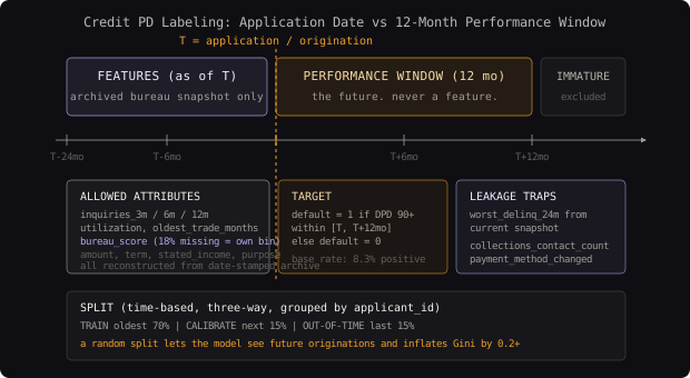
Label leakage in credit data
Credit data leaks in a way that is unusually easy to miss, because the leaked feature looks completely reasonable in a feature list.
The classic failure is a bureau attribute like worst_delinquency_24m pulled from the current bureau snapshot rather than the archived snapshot from the application date. For an account that defaulted eight months after origination, the current snapshot already contains that default. The feature is now a partial copy of the label. Models built this way routinely report Gini above 0.85 in development and collapse to 0.30 in production, and the collapse is discovered only after a full quarter of bookings.
The second failure is subtler and lives inside internal data. Fields like collections_contact_count or payment_method_changed are populated by servicing activity that happens after origination. They are not in the bureau file, so bureau discipline does not catch them, and their correlation with default is enormous.
Any attribute whose value can change after the loan is booked is a leakage candidate. The test is not "does this feature make business sense" but "could a time machine have known this value on the application date". Run that test on every column, including the ones inherited from an existing feature store.
The third issue is not leakage but selection bias, and it is specific to lending. Labels only exist for applicants who were approved and booked. The model is trained on approvals and deployed on applications. If the previous policy declined everyone with a bureau score under 580, the training data contains almost no examples from that region, and the model’s behavior there is extrapolation rather than estimation. The honest mitigation is to restrict the scoring population to the approvable range, monitor the share of scored applications falling outside the development range, and treat any reject inference technique as an assumption to be disclosed rather than a fix.
Feature engineering with weight of evidence
Raw credit attributes are a bad fit for linear models. credit_utilization has a U-shaped relationship with default (0% utilization often signals a thin or dormant file, not a low-risk one). oldest_trade_months saturates. Roughly 18% of applicants are missing a bureau score entirely, and missingness itself is predictive.
Weight of evidence (WOE) binning solves all three at once. Each numeric attribute is discretized into monotonic bins, and each bin is replaced by the log odds ratio of goods to bads in that bin relative to the population:
WOE_bin = ln( (goods_in_bin / total_goods) / (bads_in_bin / total_bads) )Missing values become their own bin with their own WOE, so missingness is modeled rather than imputed. The U-shape gets absorbed because each bin carries its own coefficient direction. And because WOE is already on a log-odds scale, a logistic regression on WOE-transformed features is close to additive in the units the model natively speaks.
The companion measure, information value (IV), summarizes how much an attribute discriminates:
IV = sum over bins of ( (goods_in_bin/total_goods) - (bads_in_bin/total_bads) ) * WOE_binThe industry heuristic: IV under 0.02 is useless, 0.02 to 0.1 is weak, 0.1 to 0.3 is medium, 0.3 to 0.5 is strong, and above 0.5 is suspicious enough to be checked for leakage before it is celebrated.
# Monotonic WOE binning with a decision-tree split search, plus information value.
import numpy as np
import pandas as pd
from sklearn.tree import DecisionTreeClassifier


def fit_woe_bins(x: pd.Series, y: pd.Series, max_bins: int = 8, min_frac: float = 0.05):
    """Return bin edges, per-bin WOE, and the attribute's information value."""
    mask = x.notna()
    tree = DecisionTreeClassifier(
        max_leaf_nodes=max_bins,
        min_samples_leaf=max(int(min_frac * mask.sum()), 50),
        random_state=42,
    )
    tree.fit(x[mask].to_frame(), y[mask])

    thresholds = tree.tree_.threshold[tree.tree_.feature >= 0]
    edges = [-np.inf] + sorted(float(t) for t in thresholds) + [np.inf]

    total_good = float((y == 0).sum())
    total_bad = float((y == 1).sum())
    woe_map, iv = {}, 0.0

    binned = pd.cut(x, bins=edges)
    for label, idx in binned.groupby(binned, observed=True).groups.items():
        good = float((y.loc[idx] == 0).sum()) + 0.5
        bad = float((y.loc[idx] == 1).sum()) + 0.5
        dist_good, dist_bad = good / total_good, bad / total_bad
        woe = float(np.log(dist_good / dist_bad))
        woe_map[str(label)] = woe
        iv += (dist_good - dist_bad) * woe

    # Missing gets its own bin, computed the same way.
    if (~mask).any():
        good = float((y[~mask] == 0).sum()) + 0.5
        bad = float((y[~mask] == 1).sum()) + 0.5
        dist_good, dist_bad = good / total_good, bad / total_bad
        woe_missing = float(np.log(dist_good / dist_bad))
        woe_map["__missing__"] = woe_missing
        iv += (dist_good - dist_bad) * woe_missing

    return {"edges": edges, "woe": woe_map, "iv": float(iv)}
The + 0.5 on each count is Laplace smoothing on the bin, and it matters: without it, a bin containing zero defaults produces an infinite WOE, and the coefficient fitted on top of it will be nonsense.
Enforcing monotonicity is a second pass. After the tree finds candidate edges, adjacent bins whose WOE violates the expected direction are merged until the sequence is monotone. This is the step that satisfies the model review requirement that risk cannot fall as delinquency count rises.
# Merge adjacent bins until per-bin WOE is monotonic in the expected direction.
def enforce_monotonic(bin_stats: list[dict], direction: str = "decreasing") -> list[dict]:
    """bin_stats is ordered low-to-high with keys: lower, upper, good, bad, woe."""
    sign = -1.0 if direction == "decreasing" else 1.0
    bins = [dict(b) for b in bin_stats]

    changed = True
    while changed and len(bins) > 2:
        changed = False
        for i in range(len(bins) - 1):
            if sign * (bins[i + 1]["woe"] - bins[i]["woe"]) < 0:
                merged = {
                    "lower": bins[i]["lower"],
                    "upper": bins[i + 1]["upper"],
                    "good": bins[i]["good"] + bins[i + 1]["good"],
                    "bad": bins[i]["bad"] + bins[i + 1]["bad"],
                }
                total_good = sum(b["good"] for b in bins)
                total_bad = sum(b["bad"] for b in bins)
                merged["woe"] = float(
                    np.log(
                        ((merged["good"] + 0.5) / total_good)
                        / ((merged["bad"] + 0.5) / total_bad)
                    )
                )
                bins[i : i + 2] = [merged]
                changed = True
                break
    return bins
The split that this problem demands
A random split is wrong here for two independent reasons. Macroeconomic conditions shift default rates over time, so a random split lets the model see the future. And applications from the same applicant (repeat borrowers are 11% of the file) must not straddle the split.
The split is therefore time-based, three-way, with a grouped guard:
# Out-of-time split with a held-out calibration slice and no applicant straddling folds.
import pandas as pd


def split_oot(df: pd.DataFrame, app_date: str = "application_date",
              group_col: str = "applicant_id"):
    """Train on the oldest cohort, calibrate on the middle, evaluate out of time."""
    df = df.sort_values(app_date).reset_index(drop=True)
    n = len(df)
    train_end = df.loc[int(0.70 * n), app_date]
    calib_end = df.loc[int(0.85 * n), app_date]

    train = df[df[app_date] < train_end]
    calib = df[(df[app_date] >= train_end) & (df[app_date] < calib_end)]
    oot = df[df[app_date] >= calib_end]

    # A repeat applicant appearing in train must not also appear downstream.
    seen = set(train[group_col])
    calib = calib[~calib[group_col].isin(seen)]
    oot = oot[~oot[group_col].isin(seen | set(calib[group_col]))]

    return train, calib, oot
The middle slice is the calibration set, and reserving it up front is the decision that makes the rest of this post work. Calibrating on training predictions is circular, and calibrating on the out-of-time set contaminates the only honest estimate of production performance.
WOE binning is usually sold as a way to handle non-linearity. Its more valuable property is that it makes the feature space stable: bin boundaries fixed at development time mean a drifting input distribution shows up as a shifting bin population, which PSI detects directly, instead of silently moving a continuous coefficient's effective operating range.
The Naive Baseline
Two baselines, both with real numbers, because they fail in different directions.
Baseline zero: predict the majority class. Every applicant is labeled good. Accuracy is 91.7%. Gini is 0.0, recall on defaults is 0.0, and the lender approves the entire book. The only thing this baseline establishes is that accuracy is a dead metric for this problem, which is worth establishing before anyone puts it on a dashboard.
Baseline one: logistic regression on raw features with median imputation.
# Raw-feature logistic regression baseline: the thing a real model has to beat.
import numpy as np
from sklearn.compose import ColumnTransformer
from sklearn.impute import SimpleImputer
from sklearn.linear_model import LogisticRegression
from sklearn.metrics import brier_score_loss, log_loss, roc_auc_score
from sklearn.pipeline import Pipeline
from sklearn.preprocessing import OneHotEncoder, StandardScaler


def build_baseline(numeric_cols: list[str], categorical_cols: list[str]) -> Pipeline:
    pre = ColumnTransformer(
        [
            ("num", Pipeline([
                ("impute", SimpleImputer(strategy="median")),
                ("scale", StandardScaler()),
            ]), numeric_cols),
            ("cat", OneHotEncoder(handle_unknown="ignore", min_frequency=0.01),
             categorical_cols),
        ]
    )
    return Pipeline([
        ("pre", pre),
        ("clf", LogisticRegression(max_iter=2000, C=1.0, solver="lbfgs")),
    ])


def report(y_true, p_hat, label: str) -> dict:
    auc = roc_auc_score(y_true, p_hat)
    return {
        "model": label,
        "auc": round(auc, 4),
        "gini": round(2 * auc - 1, 4),
        "log_loss": round(log_loss(y_true, p_hat), 5),
        "brier": round(brier_score_loss(y_true, p_hat), 5),
        "mean_pred": round(float(np.mean(p_hat)), 4),
        "actual_rate": round(float(np.mean(y_true)), 4),
    }
On the out-of-time holdout this baseline gives Gini 0.361, log loss 0.2712, Brier 0.0698, and ECE 0.071. Mean predicted probability is 0.069 against an actual default rate of 0.083, so the model is 17% optimistic on average.
That last pair of numbers is the interesting failure. The baseline is not just weakly discriminating, it is biased low, and it is biased low in the worst possible place: the mid-risk band where most of the volume sits. Median-imputing a missing bureau score pushes 18% of applicants to the population median, which is a materially better score than thin-file applicants actually deserve. Every one of those loans gets under-priced.
Tying that back to the constraints from the framing section: Gini 0.361 means the top decile bad rate is only about 2.4x the population rate, which is too flat to build a profitable cut-off on. And an ECE of 0.071 on a book with an 8.3% base rate means the pricing engine is working from a number that is wrong by nearly a full percentage point of absolute default probability.
The baseline's real problem is not the 0.361 Gini, it is that its errors are structured. Random error averages out across a portfolio. Systematic optimism on one segment compounds, because that segment gets approved at a rate the pricing never justified.
The Solution
The approach is a WOE scorecard: monotonic WOE binning, feature selection by information value and correlation pruning, L2-regularized logistic regression on the WOE-transformed features, then an explicit calibration stage fitted on the held-out calibration slice, then a linear transform into integer points.
Why this beats two plausible alternatives, stated before the code rather than after:
- Versus raw-feature logistic regression (the baseline): WOE handles the U-shaped and saturating relationships that a linear term cannot, and it models missingness instead of imputing it away. That is worth roughly 0.19 Gini on this dataset, most of it from the bureau-score-missing population.
- Versus gradient boosting: LightGBM on the same features reaches Gini 0.612, about 0.03 higher. It cannot produce a defensible per-feature reason code without a SHAP computation that adds 4 to 8ms per request and is itself an approximation of the model rather than the model, and its raw margin output is not a calibrated probability either. On a problem where the probability must be right and the explanation must be exact, trading 0.03 Gini for both is the correct trade. If the use case were internal portfolio monitoring with no adverse action requirement, the trade would flip.
The mechanism, as an analogy before the math: a scorecard is a panel of specialists who each get a fixed number of votes. The WOE step decides what each specialist’s opinion is worth in log-odds units. The logistic regression decides how many votes each specialist gets. Nobody’s vote depends on anybody else’s, which is exactly why you can tell a declined applicant which specialist voted against them.
Feature selection
180 bureau attributes plus application fields, and many of them are near-duplicates: inquiries_3m, inquiries_6m, and inquiries_12m correlate above 0.85. Feeding all three into a logistic regression produces unstable coefficients whose signs flip between refits, which is fatal for a model that has to produce stable reason codes.
# Select by information value, then prune correlated survivors to keep coefficients stable.
import numpy as np
import pandas as pd


def select_features(woe_frame: pd.DataFrame, iv_by_feature: dict[str, float],
                    iv_floor: float = 0.02, iv_ceiling: float = 0.60,
                    corr_max: float = 0.70) -> list[str]:
    """Rank by IV, drop leakage-suspect highs, then greedily drop correlated pairs."""
    candidates = [
        f for f, iv in sorted(iv_by_feature.items(), key=lambda kv: -kv[1])
        if iv_floor <= iv <= iv_ceiling
    ]
    corr = woe_frame[candidates].corr().abs()

    kept: list[str] = []
    for feature in candidates:  # already IV-descending, so the first kept wins ties
        if all(corr.loc[feature, k] < corr_max for k in kept):
            kept.append(feature)
    return kept
The iv_ceiling of 0.60 is a leakage tripwire, not a statistical rule. In four years of this data, no legitimate single attribute reached IV 0.60. When one does, it is nearly always a post-origination field that slipped into the feature store. Flagging it for review beats discovering it in production.
This step takes 180 candidates to 22 final features.
Model and objective
# L2 logistic regression on WOE features: the scorecard core.
import numpy as np
from sklearn.linear_model import LogisticRegression


def train_scorecard(x_woe_train, y_train, c_grid=(0.01, 0.1, 1.0, 10.0),
                    x_woe_valid=None, y_valid=None):
    """Fit L2 logistic regression, picking C by validation log loss, not AUC."""
    from sklearn.metrics import log_loss

    best, best_loss = None, float("inf")
    for c in c_grid:
        model = LogisticRegression(
            penalty="l2", C=c, solver="lbfgs", max_iter=1000, random_state=42,
        )
        model.fit(x_woe_train, y_train)
        p_valid = model.predict_proba(x_woe_valid)[:, 1]
        loss = log_loss(y_valid, p_valid)
        if loss < best_loss:
            best, best_loss = model, loss

    # Sign check: on WOE features every coefficient should be negative,
    # because higher WOE means lower risk by construction.
    bad_signs = int(np.sum(best.coef_[0] > 0))
    if bad_signs:
        raise ValueError(f"{bad_signs} coefficients have the wrong sign; re-bin those features")
    return best, best_loss
Two choices in that function are the substance of the section.
The objective is log loss, also called binary cross-entropy: -[y*ln(p) + (1-y)*ln(1-p)]. It is a strictly proper scoring rule, which means it is minimized uniquely when the predicted probability equals the true conditional probability. That is not a nice-to-have property here, it is the reason log loss is the right objective and AUC-surrogate losses are the wrong one. Maximizing a ranking objective optimizes order and is completely indifferent to level, so a model trained to maximize AUC has no incentive to be calibrated at all. When the output has to be multiplied by a dollar exposure, the objective has to be proper.
Model selection is on validation log loss, not validation AUC. Choosing C by AUC reliably picks a weaker-regularized model whose ranking is marginally better and whose probabilities are worse, because strong L2 shrinkage pulls predictions toward the base rate, which improves calibration and slightly flattens discrimination. Selecting on log loss makes the tradeoff correctly.
The sign check is a cheap and unusually effective guard. On WOE-transformed features every coefficient must be negative, since higher WOE means more good-like by construction. A positive coefficient is a signal that the bin ordering is broken or that the feature is collinear with another survivor, and catching it here saves a round of model review.
Hyperparameters that actually matter:
| Hyperparameter | Value | Why |
|---|---|---|
C (inverse L2 strength) |
0.1 | Selected on validation log loss. Shrinkage stabilizes coefficients across quarterly refits, which matters more than the last 0.005 of Gini. |
max_bins per attribute |
8 | Beyond 8, bins hold under 5% of the population and their WOE estimates get noisy enough to break monotonicity on refit. |
min_frac per bin |
0.05 | Guarantees roughly 39,000 rows and about 3,200 defaults per bin at this sample size, so each WOE is estimated on enough events to be stable. |
iv_floor |
0.02 | Below this the attribute adds no discrimination and costs coefficient stability. |
corr_max |
0.70 | The threshold where coefficient signs started flipping between refits on this data. |
Calibration
The scorecard from the previous step is not yet a probability model, for two reasons. L2 regularization deliberately biases predictions toward the base rate. And the training sample’s default rate is not the production population’s default rate, because of the approval-based selection described earlier.
So the probabilities get fitted separately, on the held-out calibration slice.
# Fit and compare Platt scaling against isotonic regression on the held-out calibration set.
import numpy as np
from sklearn.isotonic import IsotonicRegression
from sklearn.linear_model import LogisticRegression
from sklearn.metrics import brier_score_loss, log_loss


def expected_calibration_error(y_true, p_hat, n_bins: int = 20) -> float:
    """Bin predictions by quantile, then average the gap between predicted and actual."""
    y_true, p_hat = np.asarray(y_true), np.asarray(p_hat)
    edges = np.quantile(p_hat, np.linspace(0, 1, n_bins + 1))
    edges[0], edges[-1] = -np.inf, np.inf
    idx = np.digitize(p_hat, edges[1:-1])

    ece = 0.0
    for b in range(n_bins):
        mask = idx == b
        if not mask.any():
            continue
        ece += (mask.mean()) * abs(p_hat[mask].mean() - y_true[mask].mean())
    return float(ece)


def fit_calibrator(p_raw_calib, y_calib, method: str = "isotonic"):
    """Map raw scorecard probabilities onto observed frequencies."""
    if method == "platt":
        logit = np.log(np.clip(p_raw_calib, 1e-6, 1 - 1e-6)
                       / (1 - np.clip(p_raw_calib, 1e-6, 1 - 1e-6)))
        cal = LogisticRegression(C=1e6, solver="lbfgs")
        cal.fit(logit.reshape(-1, 1), y_calib)
        return lambda p: cal.predict_proba(
            np.log(np.clip(p, 1e-6, 1 - 1e-6) / (1 - np.clip(p, 1e-6, 1 - 1e-6))).reshape(-1, 1)
        )[:, 1]

    iso = IsotonicRegression(out_of_bounds="clip", y_min=1e-5, y_max=1 - 1e-5)
    iso.fit(p_raw_calib, y_calib)
    return lambda p: iso.predict(p)


def calibration_slope_intercept(y_true, p_hat) -> tuple[float, float]:
    """Regress outcomes on predicted logits. Slope 1.0 and intercept 0.0 is perfect."""
    logit = np.log(np.clip(p_hat, 1e-6, 1 - 1e-6) / (1 - np.clip(p_hat, 1e-6, 1 - 1e-6)))
    fit = LogisticRegression(C=1e6, solver="lbfgs").fit(logit.reshape(-1, 1), y_true)
    return float(fit.coef_[0][0]), float(fit.intercept_[0])
Both calibrators were fitted and compared on out-of-time data:
| Calibrator | Gini | Log loss | Brier | ECE | Calibration slope |
|---|---|---|---|---|---|
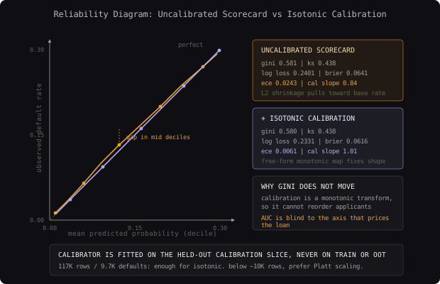
| None (raw scorecard) | 0.581 | 0.2401 | 0.0641 | 0.0243 | 0.84 |
| Platt scaling | 0.581 | 0.2338 | 0.0619 | 0.0091 | 0.99 |
| Isotonic regression | 0.580 | 0.2331 | 0.0616 | 0.0061 | 1.01 |
Isotonic wins on ECE because the miscalibration on this model is not a single global shift. It is mild optimism in the middle deciles and mild pessimism at the top, and a one-parameter sigmoid correction cannot fix a shape like that. Isotonic can, because it is a free-form monotonic map. The cost is that isotonic needs more calibration data to avoid fitting noise. At 117,000 calibration rows with roughly 9,700 defaults it is comfortable. Below about 10,000 rows, Platt is the safer choice, which is the standard finding from Niculescu-Mizil and Caruana’s 2005 comparison.
Note that Gini barely moves. Calibration is a monotonic transform, so it cannot change the ranking, and therefore cannot change AUC beyond tie-handling noise. That is exactly the point: calibration fixes the axis that AUC does not measure.
From probability to scorecard points
The last step converts calibrated probability into an integer score, which is what underwriters, policy rules, and applicants actually see.
# Convert log-odds into scorecard points using the standard PDO transform.
import numpy as np


def points_transform(base_score: int = 600, base_odds: float = 50.0, pdo: int = 20):
    """PDO is 'points to double the odds'. base_odds is good:bad at base_score."""
    factor = pdo / np.log(2.0)
    offset = base_score - factor * np.log(base_odds)
    return factor, offset


def score_from_probability(p_default: np.ndarray, base_score: int = 600,
                           base_odds: float = 50.0, pdo: int = 20) -> np.ndarray:
    factor, offset = points_transform(base_score, base_odds, pdo)
    p = np.clip(p_default, 1e-6, 1 - 1e-6)
    odds_good_bad = (1 - p) / p
    return np.round(offset + factor * np.log(odds_good_bad)).astype(int)


def attribute_points(woe_row: dict, coefficients: dict, intercept: float,
                     n_features: int, base_score: int = 600,
                     base_odds: float = 50.0, pdo: int = 20) -> dict:
    """Per-attribute points: this is the adverse action reason code."""
    factor, offset = points_transform(base_score, base_odds, pdo)
    per_feature_offset = (offset + factor * intercept) / n_features
    return {
        feature: round(per_feature_offset + factor * coefficients[feature] * woe)
        for feature, woe in woe_row.items()
    }
With pdo = 20, every 20 points doubles the good-to-bad odds. A score of 600 means 50:1 odds (about 1.96% default probability), 620 means 100:1, 580 means 25:1. Underwriters reason about this scale fluently in a way they never do about raw probabilities, and attribute_points decomposes any score into per-attribute contributions that sum exactly to the total. The five attributes with the most negative contribution are the adverse action reasons, and they are exact rather than attributed.
The single decision that mattered most was reserving a calibration slice before any modeling started. Everything else here is standard scorecard practice. Without that slice there is no honest way to fit the probability mapping, and the model ends up either circularly calibrated on its own training predictions or calibrated on the holdout that was supposed to be the unbiased estimate.
Evaluation and Metrics
Credit risk evaluation splits cleanly into two questions that need different metrics, and conflating them is how models pass review and lose money.
Discrimination: can the model separate goods from bads? The industry metric is Gini, 2 * AUC - 1, reported alongside the KS statistic, the maximum vertical gap between the cumulative distributions of goods and bads. KS is popular in lending because it points directly at the score region where separation is strongest, which is where a cut-off should sit.
Calibration: are the predicted probabilities right in absolute terms? Brier score (mean squared error on probabilities), ECE (population-weighted average gap between predicted and observed rates per bin), and calibration slope and intercept from regressing outcomes on predicted logits.
Why not accuracy: at an 8.3% base rate, predicting every applicant good scores 91.7%. Why not ROC-AUC alone: ROC-AUC is invariant to any monotonic transform of the score, so it literally cannot detect the miscalibration that drives the pricing error. Why not PR-AUC as the headline: PR-AUC is the right choice when the positive class is rare and the cost is concentrated in a small flagged set, as in fraud. Here 8.3% is imbalanced but not extreme, decisions are made across the whole score range rather than on a small flagged tail, and Gini is what regulators, rating agencies, and every vendor benchmark report in.
# Full evaluation: discrimination, calibration, and the decile table underwriting reads.
import numpy as np
import pandas as pd
from sklearn.metrics import brier_score_loss, log_loss, roc_auc_score, roc_curve


def ks_statistic(y_true, p_hat) -> float:
    fpr, tpr, _ = roc_curve(y_true, p_hat)
    return float(np.max(tpr - fpr))


def evaluate(y_true, p_hat, label: str) -> dict:
    auc = roc_auc_score(y_true, p_hat)
    slope, intercept = calibration_slope_intercept(y_true, p_hat)
    return {
        "model": label,
        "gini": round(2 * auc - 1, 4),
        "ks": round(ks_statistic(y_true, p_hat), 4),
        "log_loss": round(log_loss(y_true, p_hat), 5),
        "brier": round(brier_score_loss(y_true, p_hat), 5),
        "ece": round(expected_calibration_error(y_true, p_hat), 5),
        "cal_slope": round(slope, 3),
        "cal_intercept": round(intercept, 3),
    }


def decile_table(y_true, p_hat) -> pd.DataFrame:
    """Risk deciles with predicted vs actual rates. The calibration check by segment."""
    df = pd.DataFrame({"y": np.asarray(y_true), "p": np.asarray(p_hat)})
    df["decile"] = pd.qcut(df["p"], 10, labels=False, duplicates="drop")
    out = df.groupby("decile").agg(
        n=("y", "size"),
        predicted_rate=("p", "mean"),
        actual_rate=("y", "mean"),
        bads=("y", "sum"),
    )
    out["lift"] = out["actual_rate"] / df["y"].mean()
    out["cum_bad_capture"] = (
        out["bads"][::-1].cumsum()[::-1] / out["bads"].sum()
    )
    out["cal_gap"] = out["predicted_rate"] - out["actual_rate"]
    return out.round(4)
Out-of-time results across the three models:
| Model | Gini | KS | Log loss | Brier | ECE | Cal. slope |
|---|---|---|---|---|---|---|
| Majority class | 0.000 | 0.000 | 0.2891 | 0.0761 | 0.0000 | n/a |
| Raw logistic regression | 0.361 | 0.281 | 0.2712 | 0.0698 | 0.0710 | 0.72 |
| WOE scorecard (uncalibrated) | 0.581 | 0.438 | 0.2401 | 0.0641 | 0.0243 | 0.84 |
| WOE scorecard + isotonic | 0.580 | 0.438 | 0.2331 | 0.0616 | 0.0061 | 1.01 |
The two rows that tell the story are the last two. Gini is flat and ECE drops by 4x. That is a change no ranking metric can see and every pricing model feels.
The decile table on the final model:
| Decile | n | Predicted rate | Actual rate | Lift | Cum. bad capture |
|---|---|---|---|---|---|
| 0 (safest) | 11,700 | 0.0121 | 0.0114 | 0.14 | 1.000 |
| 3 | 11,700 | 0.0398 | 0.0411 | 0.50 | 0.906 |
| 6 | 11,700 | 0.0891 | 0.0874 | 1.05 | 0.679 |
| 8 | 11,700 | 0.1642 | 0.1689 | 2.03 | 0.402 |
| 9 (riskiest) | 11,700 | 0.2814 | 0.2771 | 3.34 | 0.223 |
Every decile’s predicted rate sits within 0.005 of its actual rate, which is the practical definition of a calibrated model. The riskiest decile carries 3.34x the population default rate and accounts for 22.3% of all defaults.
The signal that catches a silent production regression is the calibration gap in the highest risk decile, tracked by origination vintage. Overall ECE can stay flat while the top decile drifts, because the top decile is 10% of volume and its error gets averaged away. That decile is also where nearly all the loss lives, so a 3-point gap there costs more than a 0.02 Gini drop anywhere else.
Common Pitfalls and Failure Modes
| Pitfall | Why It Happens | How to Detect | How to Fix |
|---|---|---|---|
| Post-origination leakage | Bureau or servicing attributes pulled from the current snapshot rather than the archived application-date snapshot | Single-attribute IV above 0.60, or development Gini above 0.75 on unsecured consumer credit | Rebuild every feature from date-stamped archives; add an automated as-of assertion in the feature pipeline |
| Immature accounts labeled good | The most recent 12 to 14 months have no matured outcome, and dropping them feels like throwing away the freshest data | Default rate declining monotonically with origination month in the training set | Exclude accounts whose performance window has not closed; never label them 0 |
| Selection bias from past policy | Only approved applicants have labels, so the declined region is unobserved | Compare the score distribution of all applications against the development sample; watch the share outside the development range | Restrict scoring to the approvable range, monitor out-of-range share, disclose any reject inference as an assumption |
| Calibration drift | Macro conditions move the base rate while the score ranking stays valid | Actual-versus-predicted rate by monthly vintage, and calibration intercept tracked over time | Refit the calibration intercept monthly on recent matured data; keep coefficients frozen until the annual refit |
| Population drift | The applicant mix changes through a new marketing channel or partner | PSI above 0.10 on the score distribution, or above 0.25 on individual attribute bin populations | Investigate the source channel first; refit only if the shift is structural rather than a mix effect |
| Unstable coefficients across refits | Correlated attributes survive selection and split the same signal between them | Coefficient sign flips or magnitude changes above 40% between quarterly refits | Tighten corr_max, increase L2 shrinkage, and freeze the attribute list between scheduled refits |
| Overfitted WOE bins | Bins too narrow, so per-bin WOE is estimated on too few defaults | Non-monotonic WOE reappearing after refit, or bins holding under 3% of the population | Raise min_frac, cap max_bins at 8, always run the monotonicity merge |
The mistake that sinks the most first credit models is a random train/test split. It produces a Gini in the 0.70s, everyone celebrates, and the model loses 0.25 Gini in its first production quarter. Credit data is non-stationary by construction, so a random split lets the model learn from applications that were originated after the ones it is being tested on. The out-of-time split is not a refinement of the evaluation; it is the only evaluation that means anything.
Scaling and Productionizing
A scorecard is cheap to serve and expensive to govern, which is the opposite of the usual ML cost profile.
Serving. The scored artifact is a lookup: bin the 22 attributes against fixed edges, sum 22 coefficients, apply the isotonic map, apply the points transform. Serialized, this is under 40KB of JSON, and it does not need a Python runtime.
Per-request budget (p99 target 10ms):
  bin 22 attributes against fixed edges    0.08 ms
  sum 22 coefficient contributions         0.01 ms
  isotonic lookup (200-point step fn)      0.01 ms
  points transform + reason code sort      0.04 ms
  ------------------------------------------------
  model compute                            0.14 ms
  feature assembly from bureau payload     1.9  ms
  serialization + network in-cluster       2.1  ms
  ------------------------------------------------
  total p99                                4.2  ms
The model is 3% of the latency budget. Feature assembly is the real cost, which is the normal shape for tabular credit models and the reason “make the model faster” is almost never the right optimization here.
Retraining cadence is three-tiered, and the tiering matters more than the frequency:
- Monthly: recalibrate only. Refit the isotonic map (or just the calibration intercept) on the most recent matured vintages. Coefficients stay frozen. This tracks base rate movement without disturbing the reason codes or the score distribution, so no policy change is required.
- Quarterly: monitor, do not refit. PSI on the score and on every attribute’s bin population, decile calibration gaps by vintage, coefficient drift if a shadow refit is run.
- Annually: full refit. Re-bin, re-select, re-fit, re-calibrate, and take it through model review. Anything more frequent than annual makes the score non-comparable across vintages, which breaks the policy cut-offs the business has already set.
Feature freshness is a hard dependency on the bureau. A stale bureau pull, even 48 hours old, can miss a new delinquency. The pipeline enforces a maximum pull age and fails closed to manual underwriting rather than scoring on stale data.
The monitoring signal for silent degradation is the vintage calibration curve: for each origination month, the predicted default rate at booking against the actual rate observed as that vintage matures. Because labels lag 12 months, this is watched at intermediate milestones too (30+ DPD at month 3, 60+ DPD at month 6) as early indicators. The specific pattern that means trouble is the actual rate exceeding predicted for three consecutive vintages at the same maturity milestone. Discrimination, measured by Gini, usually holds up for years. Calibration goes first, and it goes quietly, because nothing in the ranking metrics moves at all.
Separating monthly recalibration from annual refitting is what makes a scorecard survive in production. Calibration drifts with the economy and can be corrected with a one-parameter update that nobody has to review. Discrimination drifts with the applicant population and needs a full refit. Treating them as one maintenance task means either over-refitting a stable model or under-correcting a drifting probability.
This is essentially the FICO scorecard methodology, in production across the consumer lending industry since the late 1950s and still the reference approach: binned attributes, additive points, explicit reason codes. The calibration layer is where modern practice diverges. Platt scaling comes from Platt's 1999 work on probabilistic SVM outputs, and the isotonic alternative from Zadrozny and Elkan's 2002 paper; Niculescu-Mizil and Caruana's 2005 comparison is the standard reference for when to prefer each. Upstart's SEC filings describe gradient-boosted risk models with an explainability layer on top, which is the same tradeoff resolved in the other direction for a lender whose regulatory posture supports it.
Alternative Approaches
| Approach | Gini (OOT) | ECE after calibration | Training cost | Interpretability | Best fit |
|---|---|---|---|---|---|
| Raw logistic regression | 0.361 | 0.038 | Seconds | High, but coefficients on raw units mislead when relationships are non-monotonic | A first baseline, nothing more |
| WOE scorecard + isotonic | 0.580 | 0.006 | About 4 min on 780K rows | Highest: exact additive points, reason codes sum to the score | Regulated consumer lending with adverse action requirements |
| LightGBM + isotonic | 0.612 | 0.008 | About 12 min on 780K rows | Low: needs SHAP, which approximates the model rather than decomposing it | Portfolio monitoring, collections prioritization, any internal-only use |
| Explainable boosting machine (GA2M) | 0.598 | 0.007 | About 45 min on 780K rows | Medium-high: additive shape functions plus selected pairwise interactions | A middle path when review accepts shape functions over points |
| Neural network (3 hidden layers) | 0.589 | 0.011 | About 25 min on GPU | Very low | Hard to justify: worse than boosting and far less explainable |
For a regulated consumer lender, the WOE scorecard with isotonic calibration is the model to ship, and the 0.03 Gini gap to LightGBM is a real cost paid for a real requirement. Exact reason codes, a score distribution that is stable enough to set policy on for a year, a 40KB artifact with no Python dependency at serving time, and a model review process that a credit risk committee can complete in a single session are together worth more than 0.03 Gini.
The point at which that flips is when the adverse action requirement disappears. For a collections prioritization model or an internal portfolio stress model, nobody is entitled to an explanation, and LightGBM plus isotonic is straightforwardly better. The explainable boosting machine is the genuinely interesting middle option and is gaining ground in credit: it recovers most of the boosting lift while keeping an additive structure that review can reason about. It is not yet the default because points-based scorecards have fifty years of regulatory precedent and shape functions do not.
Key Takeaways
- Calibration and discrimination are orthogonal. A monotonic transform cannot change AUC and can cut ECE by 4x. If you only report ranking metrics, you have no visibility into the axis that sets the price.
- Log loss is a proper scoring rule and AUC is not. Train and select on log loss when the output must be a probability. Selecting
Con AUC reliably picks a worse-calibrated model. - WOE binning earns its place by absorbing non-monotonicity, modeling missingness, and stabilizing the feature space. The third property is the underrated one, because it makes drift detectable as a bin population shift.
- Reserve a calibration slice before you start. Calibrating on training predictions is circular and calibrating on the holdout destroys the only honest performance estimate.
- Time-based splits are mandatory in credit, not a refinement. Random splits inflate Gini by 0.2 or more and the inflation is invisible until production.
- Immature accounts must be excluded, never labeled good. Labeling them 0 teaches the model that recent originations are safe, which is the exact opposite of what a risk model should learn.
- Isotonic beats Platt when miscalibration has shape, and needs about 10,000 calibration rows to earn that. Below that, the one-parameter sigmoid is safer.
- Separate monthly recalibration from annual refitting. The economy moves calibration; the applicant population moves discrimination. Different problems, different cadences, different review burdens.
The counter-intuitive lesson is that the best model here is deliberately the more regularized one. C = 0.1 gave slightly worse validation AUC than C = 1.0 and was selected anyway, because the shrinkage that flattens discrimination is the same shrinkage that stabilizes coefficients across refits and keeps predictions near the base rate where calibration is easiest to maintain. In a domain where the model has to produce the same reason codes next quarter and the same score distribution next year, stability is a performance metric. Most tabular ML tuning advice implicitly assumes it is not.
Frequently Asked Questions
Q: Why not just use gradient boosting and add SHAP for explanations?
A: SHAP values approximate a feature’s contribution by averaging over coalitions; they are not a decomposition of the model’s actual computation. For adverse action reasons, “this attribute cost you 34 points, and the 22 attribute contributions sum exactly to your score” is a defensible statement in a way that “SHAP attributes 0.031 of log-odds to this attribute under the TreeSHAP background distribution” is not. There is also a 4 to 8ms per-request cost. When the regulatory requirement is absent, boosting plus isotonic is the better model.
Q: Why isotonic regression instead of Platt scaling?
A: The miscalibration on this model has shape rather than a single global offset: mild optimism in the middle deciles, mild pessimism at the top. Platt scaling is a one-parameter sigmoid correction and structurally cannot fix that, which is why it lands at ECE 0.0091 against isotonic’s 0.0061. The tradeoff is data hunger. With fewer than roughly 10,000 calibration rows, isotonic starts fitting noise and Platt becomes the safer choice.
Q: Why is ECE the guardrail metric rather than Brier score?
A: Brier score is a proper scoring rule but it mixes discrimination and calibration into one number, so a model can improve its Brier score by ranking better while calibrating worse. ECE isolates calibration by construction: it bins predictions and averages the gap between predicted and observed frequency. Since discrimination is already tracked by Gini, the guardrail should measure only the thing Gini cannot see. Both get reported; ECE is the one with a threshold attached.
Q: Why not oversample defaults or use class weights, given the 8.3% imbalance?
A: Because both destroy calibration, which is the property the model exists to provide. Oversampling shifts the implied prior and makes every predicted probability too high by a factor you then have to undo analytically. At 8.3% positives with 64,700 default events, there is no estimation problem that resampling would solve. Resampling earns its place at base rates under roughly 1%, and even then the probabilities need correcting afterward.
Q: How do you handle a new attribute that only exists for recent applications?
A: You do not add it to the production scorecard until it has 12 months of matured performance behind it, because binning it on a partial window produces WOE estimates from a non-random slice of outcomes. In the interim it can run in a shadow model whose predictions are logged but not used. The alternative, treating the historical absence as a missing-value bin, conflates “attribute did not exist” with “attribute is unavailable for this applicant”, and those two carry completely different risk signals.
Q: What breaks first when this model degrades in production?
A: Calibration, and it breaks silently. Gini on this scorecard family typically holds within 0.03 for two to three years, because the relative ordering of credit risk is remarkably stable. The absolute default rate moves with unemployment, rate cycles, and the lender’s own marketing mix, so the predicted-versus-actual gap opens well before any ranking metric twitches. That is why the vintage calibration curve at intermediate DPD milestones is the primary monitoring surface, not the Gini dashboard.
Interview Questions
Q: Your model has an AUC of 0.79 and a mean predicted probability of 6% against an observed default rate of 9%. What is wrong, and how would you fix it without retraining?
Expected depth: Identify this as pure miscalibration with intact discrimination. Explain that AUC is invariant to monotonic transforms so it cannot detect this. Propose fitting a calibration map on held-out matured data, Platt versus isotonic depending on whether the error is a global shift or has shape, and note that an intercept-only correction suffices if the gap is uniform across deciles. Mention checking whether the gap is uniform via a decile table before choosing.
Q: Explain weight of evidence and information value. Why transform features this way instead of one-hot encoding or splining them?
Expected depth: Give both formulas. Explain that WOE puts every bin on a log-odds scale, which matches the logistic link, so coefficients stay interpretable and the model stays additive. Cover the three practical wins: non-monotonic relationships like U-shaped utilization, missingness as an explicit modeled bin, and bin-population drift being directly measurable by PSI. Contrast with one-hot, which loses ordering and explodes dimensionality, and splines, which handle non-linearity but do not give you a points decomposition.
Q: Why is log loss the right training objective here when the business metric is Gini?
Expected depth: Define a strictly proper scoring rule and state that log loss is minimized uniquely at the true conditional probability. Explain that ranking objectives are invariant to level, so optimizing them gives the model no incentive toward calibration. Connect to EL = PD * LGD * EAD: the output is multiplied by a dollar exposure, so level errors translate directly into mis-pricing. Note the practical consequence that hyperparameter selection on AUC picks a worse-calibrated model than selection on log loss.
Q: You are handed a credit model with a development Gini of 0.82 on unsecured consumer loans. What is your first hypothesis?
Expected depth: Leakage, specifically post-origination information. Name the two likely mechanisms: bureau attributes pulled from a current snapshot rather than the archived application-date snapshot, and internal servicing fields such as collections contacts that only populate after booking. Add a random rather than out-of-time split as a second hypothesis. Describe the diagnostic: rank attributes by IV and inspect anything above 0.5, then audit the as-of timestamp on the top contributors. Anchor with a realistic range: 0.45 to 0.65 Gini is normal for this product.
Q: Only approved applicants have performance labels. How does that bias the model, and what would you do about it?
Expected depth: Name it as selection bias or sample selection on the outcome, not covariate shift. Explain that the training population is censored by the prior policy, so the model extrapolates rather than estimates in the declined region. Discuss reject inference options and their assumptions: parcelling, augmentation, fuzzy augmentation, and bivariate probit with an exclusion restriction, noting that all of them assume something unverifiable about the unobserved outcomes. Argue for the honest operational answer: restrict scoring to the approvable range, monitor the share of applications falling outside the development range, and use controlled random-approval test cells to generate genuinely unbiased labels in the boundary region if the business will fund them.
View full code for this problem