Build a Loan Default Predictor with XGBoost and SHAP Explainability
classical-ml model-evaluation feature-engineering mlops View full code for this problem
ML Problem & Solution
Loan Default Prediction with XGBoost and SHAP
A model that beats the scorecard is worthless if you cannot tell an applicant why they were declined
A lender originates 38,000 unsecured personal loans a quarter, 3,000 to 35,000 dollars each, 24 to 60 month terms. About 7.4% of them go 90 days past due within the first year. Each of those costs the lender 61% of the outstanding principal after recoveries, which on a 14,200 dollar average balance is roughly 8,700 dollars. The existing decision engine is a logistic-regression scorecard built on weight-of-evidence bins, refreshed every 18 months, and it has a Gini coefficient of 0.41.
The obvious move is to replace the scorecard with gradient boosting and collect the lift. That works, and it takes about a day. The reason it usually does not ship is the second requirement, which nobody mentions in the first meeting: under the Equal Credit Opportunity Act and Regulation B in the United States, a declined applicant is entitled to a statement of the specific principal reasons for the denial. Similar obligations exist in the EU under GDPR Article 22 and in the UK under FCA consumer credit rules. A scorecard produces those reasons for free, because the score is a sum of signed points per bin and the reasons are the bins that cost the applicant the most points. A gradient-boosted tree ensemble with 1,400 trees and depth-6 interactions produces a number, and a global feature importance chart, and nothing you can put in a letter.
So the actual problem is a joint one. Improve discrimination enough to be worth a model-risk review, and produce a per-decision attribution that is faithful to the model, stable across retrains, consistent with the direction of the applicant’s own values, and cheap enough to compute for every one of 38,000 quarterly decisions plus the declined applications on top. That is what SHAP is for, and the interesting part is not calling shap.TreeExplainer, which takes one line. It is what happens when the attributions disagree with the credit policy team’s intuition, and which of the two is wrong.
There is also a data problem that makes loan default harder than it looks: the training data is the output of the previous model. Every applicant in the dataset with a known outcome is one the old scorecard approved. The rejected 31% have no repayment history at all, so the model learns the default behaviour of a population that has already been filtered for low risk by a different model. Its ranking is unbiased only on the approved region of the feature space, and the moment you use it to approve applicants the scorecard would have declined, you are extrapolating.
Think of it as hiring: you can only measure job performance for people you hired, so every model you build learns from a population your previous hiring rule selected. The people you rejected might have been excellent, and no amount of model tuning tells you.
Given an applicant’s credit bureau attributes, application-form fields, and bank-transaction aggregates available at underwriting time, predict the probability of 90-plus-day delinquency within 12 months of origination, optimizing Gini on the approved population, subject to producing a ranked, faithful, per-applicant reason set for every decline.
Framing the Problem
This is binary classification with a 12-month outcome window and a regulatory explainability constraint. The explainability constraint is not a nice-to-have bolted on at the end; it eliminates several otherwise reasonable model classes and it shapes the feature set, so it belongs in the framing.
The target is default_12m: the loan reached 90 days past due, was charged off, or entered a bankruptcy proceeding within 365 days of origination. Loans that prepaid in full are negatives. Loans still in a 30-or-60-day delinquency bucket at the 365-day mark are excluded, not labeled negative, which is a choice worth defending: they are 2.1% of the book, their eventual outcome is roughly 50/50, and labeling them either way injects a systematic error into exactly the region of the score distribution where the cutoff sits.
Performance window and label lag. A loan originated today cannot be labeled for 12 months. Combined with the 24-to-60-month terms, this means the most recent 12 months of originations are unlabeled, and the newest fully labeled cohort was underwritten under a slightly different policy. Every model in credit risk is trained on a world that no longer exists, and the discipline is to measure how much that matters rather than pretend it does not.
Constraints
- Adverse action reasons: every decline must produce 3 to 4 ranked principal reasons, mapped to a fixed set of 27 approved reason texts. Free-form or feature-name-based reasons are not acceptable.
- Latency: 300ms p95 for score plus attribution. Underwriting is a synchronous API call in the application flow.
- Model risk governance: the model needs documented stability (PSI under 0.10 on the score at 12 months), monotonic behaviour on 9 policy-designated features, and a champion-challenger comparison against the incumbent scorecard.
- Fair lending: disparate impact tested on the standard protected classes via proxy methods, with an adverse impact ratio above 0.80 at the production cutoff.
- No prohibited features: no direct or proxy use of protected attributes. This rules out some genuinely predictive features (postcode-level aggregates are the recurring argument).
Credit risk reports Gini (equivalently 2 * AUC - 1) because the decision is a ranking followed by a policy cutoff, and the cutoff moves with risk appetite and funding cost rather than with the model. The guardrail that actually gates deployment is different: the Kolmogorov-Smirnov statistic in the cutoff region plus calibration error in the three deciles around the cutoff, because a model with excellent overall Gini and poor separation exactly where the line is drawn buys nothing.
Guardrail metrics: score PSI under 0.10 against the development sample, adverse impact ratio above 0.80, approval rate within 2 percentage points of plan at the chosen cutoff, and expected loss rate on the approved book. Out of scope here: loss given default and exposure at default models (this post predicts probability of default only), pricing and risk-based interest assignment, and collections optimization after delinquency.
Explainability is a modeling constraint, not a reporting step. Deciding up front that every decline needs a faithful per-applicant reason set rules out stacked ensembles and blended scores, forces monotonic constraints on policy features, and changes how you encode categoricals. Retrofitting it after the model is built is where credit risk projects die.
Data and Features
The development sample is 312,000 originated loans across 14 quarterly cohorts, with 23,100 defaults, a 7.4% rate. Three sources:
| Source | Count | Examples | Notes |
|---|---|---|---|
| Credit bureau pull | 214 attributes | util_revolving, inq_6m, worst_delinq_24m, trade_lines_open, oldest_trade_months |
Strongest family. Snapshot as of the application date, not today. |
| Application form | 19 fields | stated_income, employment_months, loan_purpose, requested_amount, term_months |
Self-reported, so partly unverified and partly gameable. |
| Bank transaction aggregates | 46 features | avg_balance_90d, nsf_count_90d, income_deposit_regularity, debt_service_to_deposit |
Available on 68% of applicants via open banking consent; missingness is informative. |
Feature engineering in credit risk looks different from most tabular ML because half the work is making features defensible rather than predictive.
# Credit-risk feature construction: ratios, capped trends, and explicit missingness.
import numpy as np
import pandas as pd

def build_credit_features(df: pd.DataFrame) -> pd.DataFrame:
    out = df.copy()

    # Ratios, because absolute balances mean nothing without capacity.
    out["dti"] = out["monthly_debt_payment"] / out["stated_monthly_income"].clip(lower=500)
    out["payment_to_income"] = out["estimated_payment"] / out["stated_monthly_income"].clip(lower=500)
    out["util_revolving"] = (out["revolving_balance"] / out["revolving_limit"].clip(lower=1)).clip(0, 2.0)
    out["loan_to_income"] = out["requested_amount"] / (out["stated_monthly_income"] * 12).clip(lower=6000)

    # Trend features: recent behaviour against the applicant's own baseline.
    out["util_trend_6m"] = out["util_revolving"] - out["util_revolving_6m_ago"]
    out["inq_velocity"] = out["inq_3m"] / out["inq_12m"].clip(lower=1)

    # Missingness is informative and must be explicit, never imputed away.
    out["has_open_banking"] = out["avg_balance_90d"].notna().astype("int8")
    out["thin_file"] = (out["trade_lines_open"].fillna(0) < 3).astype("int8")

    # Cap rather than clip to NaN: a 900% utilisation is real, and an outlier at that
    # magnitude dominates a split without adding information beyond "very high".
    for col, cap in [("inq_6m", 20), ("worst_delinq_24m", 120), ("nsf_count_90d", 15)]:
        out[col] = out[col].clip(upper=cap)
    return out
XGBoost handles NaN natively by learning a default direction per split, which is the right behaviour here: an applicant with no open-banking data is a different population, and imputing their average balance to the median actively destroys signal. We do not impute. We add the indicator and let the trees route.
The leakage risk specific to loan default
The one that catches people is post-origination data in the bureau attributes. If the bureau file is refreshed on a schedule and the feature store stores the latest pull rather than the pull as of the application date, then for a loan originated 8 months ago the “current” number of delinquent trade lines includes the delinquency on this very loan. Offline Gini jumps to 0.79, the model looks spectacular, and it is reading the answer. The tell is that a single attribute like delinq_trades_now shows an enormous gain importance and a monotonic relationship that is too clean.
# Point-in-time correctness check: every feature timestamp must precede origination.
def assert_point_in_time(df: pd.DataFrame, feature_ts_cols: list[str]) -> None:
    """Fail loudly when any feature was observed after the loan was originated."""
    orig = pd.to_datetime(df["origination_date"])
    for col in feature_ts_cols:
        observed = pd.to_datetime(df[col])
        violations = int((observed > orig).sum())
        if violations:
            raise AssertionError(
                f"{col}: {violations:,} rows observed after origination. "
                "The feature store is serving the latest snapshot, not the as-of snapshot."
            )

assert_point_in_time(dev, ["bureau_pull_ts", "open_banking_pull_ts", "application_ts"])
The second leakage source is subtler and specific to self-reported fields. stated_income is captured at application, but some lenders overwrite it during verification, which happens after approval. A verified income field is not available at decision time for the applicants you declined, so training on it produces a model that cannot be deployed.
Building the training sample from the loan servicing table instead of the application table. The servicing table only contains approved and funded loans, so you silently lose the declined population, the approved-but-not-taken population (roughly 19% of approvals here), and any record of what the applicant looked like at decision time versus after verification. Always build from the application snapshot and join outcomes onto it.
Splitting by cohort, not at random
Credit data is strongly non-stationary: macro conditions, policy changes, and channel mix all shift quarterly. We split by origination cohort so the test set is genuinely out-of-time, and we keep a second out-of-time slice for the model risk validation team that no one on the modeling side is allowed to look at.
# Out-of-time cohort split. Random splits overstate credit model performance by 0.03-0.06 Gini.
COHORTS = sorted(dev["origination_quarter"].unique())

train_cohorts = COHORTS[:9]      # 2022Q1 to 2024Q1
valid_cohorts = COHORTS[9:11]    # 2024Q2 to 2024Q3, used for early stopping and tuning
oot_cohorts = COHORTS[11:13]     # 2024Q4 to 2025Q1, reported performance
locked_cohorts = COHORTS[13:]    # 2025Q2, opened once, by validation only

train = dev[dev["origination_quarter"].isin(train_cohorts)]
valid = dev[dev["origination_quarter"].isin(valid_cohorts)]
oot = dev[dev["origination_quarter"].isin(oot_cohorts)]

for name, frame in [("train", train), ("valid", valid), ("oot", oot)]:
    print(f"{name:<6} {len(frame):>7,} loans  {frame['default_12m'].mean():.2%} default  "
          f"{frame['origination_quarter'].min()} to {frame['origination_quarter'].max()}")
On our data the random-split Gini was 0.613 and the out-of-time Gini was 0.578. That 0.035 gap is the honest cost of non-stationarity, and reporting the random-split number to a model risk committee is how a model gets rejected on its second review rather than its first.
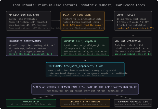
Reject inference is the elephant in this section. The model only ever learns from applicants the previous policy approved, so its ranking is trustworthy inside the approved region and speculative outside it. The practical answer is not a clever statistical correction, it is to buy the data: approve a small random sample above the cutoff (we run 1.5% of near-cutoff declines as a paid learning portfolio) and treat those loans as the cost of knowing.
The Naive Baseline
The incumbent scorecard is the baseline, and it is a strong one. That matters, because a lot of write-ups compare gradient boosting against a deliberately weak linear model and claim a large lift.
# Baseline: WOE-binned logistic regression, the standard credit scorecard construction.
import numpy as np
import pandas as pd
from sklearn.linear_model import LogisticRegression
from sklearn.metrics import roc_auc_score

def woe_transform(x: pd.Series, y: pd.Series, n_bins: int = 8) -> tuple[pd.Series, pd.DataFrame]:
    """Weight of evidence per bin: log(share of goods / share of bads)."""
    bins = pd.qcut(x, n_bins, duplicates="drop")
    table = pd.DataFrame({"bin": bins, "y": y}).groupby("bin", observed=True)["y"].agg(["count", "sum"])
    table["bad"] = table["sum"] / max(y.sum(), 1)
    table["good"] = (table["count"] - table["sum"]) / max((1 - y).sum(), 1)
    table["woe"] = np.log(table["good"].clip(lower=1e-6) / table["bad"].clip(lower=1e-6))
    return bins.map(table["woe"]).astype(float), table

SCORECARD_FEATURES = ["util_revolving", "inq_6m", "worst_delinq_24m", "dti",
                      "oldest_trade_months", "trade_lines_open", "payment_to_income"]

X_train = pd.DataFrame({c: woe_transform(train[c], train["default_12m"])[0]
                        for c in SCORECARD_FEATURES})
scorecard = LogisticRegression(max_iter=2000, C=1.0)
scorecard.fit(X_train.fillna(0.0), train["default_12m"])

auc = roc_auc_score(oot["default_12m"], scorecard.predict_proba(X_oot.fillna(0.0))[:, 1])
print(f"scorecard OOT Gini: {2 * auc - 1:.4f}")
Output: scorecard OOT Gini: 0.4112.
The scorecard is insufficient for three reasons that tie back to the constraints. It cannot express interactions, and the interactions in credit risk are real and well known: high utilisation is mildly predictive on a thick file with 12 years of history and severely predictive on a thin file with 14 months, and a single linear term cannot hold both. It uses 7 features because WOE binning plus manual review does not scale past roughly 20, leaving 260 available attributes unused. And the 8-bin quantile discretisation throws away within-bin ordering, which costs roughly 0.02 Gini on its own.
At the production cutoff of 0.094 predicted default probability, the scorecard approves 69.1% of applicants and the approved book has an expected loss rate of 5.82%. That is the number the new model has to beat, at equal approval rate.
The Solution
Three components: a monotonically constrained XGBoost model, SHAP attributions computed for every decision, and a deterministic mapping from SHAP values to the 27 approved reason texts. The third one is where the engineering is.
Model: XGBoost with monotonic constraints
XGBoost with hist tree method on 312,000 rows and 279 features trains in about 90 seconds and handles the missingness natively. The part that is specific to credit risk is monotonic constraints.
Credit policy asserts that certain relationships must hold in a fixed direction: more recent delinquencies never reduce predicted risk, higher utilisation never reduces predicted risk, longer credit history never increases it. These assertions are not learned from data, they are policy, and they exist because an unconstrained model will happily learn that applicants with 11 inquiries in 6 months default slightly less than those with 9, because of a sparse region and 40 noisy observations. When that non-monotonicity reaches an adverse action letter, the lender has told an applicant they were declined for having too few credit inquiries, and now there is a regulatory problem.
# Monotonically constrained XGBoost. The constraint vector is credit policy, not a hyperparameter.
import numpy as np
import xgboost as xgb

# +1: risk must not decrease as the feature increases. -1: risk must not increase.
POLICY_MONOTONE = {
    "util_revolving": 1,
    "inq_6m": 1,
    "worst_delinq_24m": 1,
    "dti": 1,
    "payment_to_income": 1,
    "nsf_count_90d": 1,
    "oldest_trade_months": -1,
    "avg_balance_90d": -1,
    "employment_months": -1,
}

def monotone_vector(feature_names: list[str]) -> tuple[int, ...]:
    return tuple(POLICY_MONOTONE.get(name, 0) for name in feature_names)

FEATURES = [c for c in train.columns if c not in DROP_COLS]

params = dict(
    objective="binary:logistic",
    eval_metric="auc",
    tree_method="hist",
    max_depth=6,
    min_child_weight=40,
    learning_rate=0.03,
    subsample=0.8,
    colsample_bytree=0.6,
    reg_lambda=4.0,
    reg_alpha=0.5,
    gamma=0.5,
    monotone_constraints=monotone_vector(FEATURES),
    scale_pos_weight=1.0,
    n_jobs=-1,
    random_state=23,
)

dtrain = xgb.DMatrix(train[FEATURES], label=train["default_12m"], feature_names=FEATURES)
dvalid = xgb.DMatrix(valid[FEATURES], label=valid["default_12m"], feature_names=FEATURES)

booster = xgb.train(
    params, dtrain, num_boost_round=3000,
    evals=[(dtrain, "train"), (dvalid, "valid")],
    early_stopping_rounds=150, verbose_eval=200,
)
print(f"best iteration: {booster.best_iteration}")
Note what is absent: scale_pos_weight stays at 1.0. At a 7.4% positive rate the class imbalance is mild, and since we need calibrated probabilities to compare against a probability cutoff, distorting the score scale to chase a metric that does not depend on the scale is a bad trade. This is the opposite of the choice you would make at a 0.17% base rate.
The hyperparameters that matter most, with the values we landed on:
min_child_weight=40. Credit data has sparse regions (thin-file applicants with 3 inquiries and high utilisation) where small leaves fit noise. Raising this from 1 to 40 cost 0.004 in-sample Gini and gained 0.011 out-of-time, which is the trade you want.max_depth=6. Depth 4 loses the thin-file interaction; depth 10 overfits cohort-specific quirks and out-of-time Gini fell 0.008.colsample_bytree=0.6. With 279 correlated bureau attributes, aggressive column sampling decorrelates the trees and also makes SHAP attributions more stable across retrains, which turns out to matter a lot.monotone_constraints. Costs 0.006 out-of-time Gini. Buys the entire regulatory story. Pay it.
Monotonic constraints cost real accuracy and it is worth being honest about why we pay: the constraint is a hard prior that the sparse regions of the feature space are not telling us something genuine, and in credit risk that prior is almost always correct.
Attribution: SHAP
SHAP values answer one question: for this applicant, how much did each feature move the prediction away from the population average, in log-odds. The mechanism is a cooperative-game analogy. Imagine the features are players who join a coalition in a random order and each one shifts the prediction when it joins; a feature’s SHAP value is its average marginal contribution over all possible join orders. That averaging is what makes the attributions additive: they sum exactly to the difference between this prediction and the base value.
For tree ensembles, TreeSHAP (Lundberg et al., 2018) computes this exactly in polynomial time rather than by sampling, which is why SHAP is practical here and permutation importance is not.
# Exact per-applicant SHAP attributions for a tree ensemble.
import shap

explainer = shap.TreeExplainer(booster, feature_perturbation="tree_path_dependent")
shap_values = explainer.shap_values(oot[FEATURES])       # (n_rows, n_features), log-odds units
base_value = float(explainer.expected_value)

# Additivity check: this is the property the whole reason-code system rests on.
reconstructed = base_value + shap_values.sum(axis=1)
margin = booster.predict(xgb.DMatrix(oot[FEATURES], feature_names=FEATURES), output_margin=True)
assert np.abs(reconstructed - margin).max() < 1e-4, "SHAP additivity violated"
Two details matter here and both are easy to get wrong.
feature_perturbation="tree_path_dependent" uses the tree structure’s own coverage statistics and needs no background dataset. The alternative, "interventional", requires a background sample and gives values that are causally cleaner but depend on which background you chose, which means the reason an applicant received can change because someone resampled the background set. For adverse action reasons, reproducibility beats causal purity, so tree_path_dependent is the right default.
SHAP values are in log-odds, not probability. A SHAP value of +0.8 on util_revolving means that feature pushed the applicant 0.8 log-odds toward default relative to the base rate. Do not convert individual SHAP values to probability deltas; the transform is nonlinear so the parts stop summing to the whole.
Reason codes: the part that is actually hard
The naive implementation takes the top 4 SHAP values and emits their feature names. This fails immediately in four ways, and the fixes are the real content of this section.
First, engineered features are not explainable to a human. inq_velocity is a ratio of two inquiry counts; “your inquiry velocity was too high” is not a reason anyone can act on. So features are grouped into reason families, and the SHAP values within a family are summed. Additivity is what makes this legitimate: the sum of SHAP values over a group is the group’s contribution, exactly.
Second, a feature can push toward default for a reason that is not the applicant’s fault in the direction you think. Only positive contributions (toward default) are eligible as decline reasons, and only when the applicant’s own value is on the adverse side of the population median for that family. A family with a positive SHAP value but a favourable raw value indicates a model interaction, not an applicant deficiency, and putting it in a letter is indefensible.
Third, the reasons must be stable. If two retrains a month apart give the same applicant a different top reason, the lender has an audit problem. Families are coarser than features and therefore far more stable: measured across 12 monthly retrains, the top feature changed for 31% of declined applicants and the top family changed for 6%.
Fourth, the ranked families must map to the 27 pre-approved reason texts, which is a fixed lookup reviewed by legal.
# SHAP values to ranked adverse action reasons. Family grouping is what makes this defensible.
import numpy as np
import pandas as pd

REASON_FAMILIES = {
    "delinquency_history": ["worst_delinq_24m", "delinq_trades_24m", "months_since_delinq"],
    "credit_utilisation": ["util_revolving", "util_revolving_6m_ago", "util_trend_6m",
                           "revolving_balance"],
    "recent_credit_seeking": ["inq_3m", "inq_6m", "inq_12m", "inq_velocity", "new_trades_6m"],
    "debt_burden": ["dti", "payment_to_income", "loan_to_income", "monthly_debt_payment"],
    "credit_history_length": ["oldest_trade_months", "avg_trade_age_months", "thin_file"],
    "cash_flow": ["avg_balance_90d", "nsf_count_90d", "debt_service_to_deposit",
                  "income_deposit_regularity"],
    "employment_stability": ["employment_months", "employment_type"],
}

REASON_TEXT = {
    "delinquency_history": "Serious delinquency on your credit report",
    "credit_utilisation": "Proportion of revolving balances to credit limits is too high",
    "recent_credit_seeking": "Too many recent inquiries or newly opened accounts",
    "debt_burden": "Level of existing debt relative to income",
    "credit_history_length": "Length of credit history is insufficient",
    "cash_flow": "Insufficient or irregular deposit activity in linked accounts",
    "employment_stability": "Length of employment",
}

def adverse_action_reasons(
    shap_row: np.ndarray,
    feature_values: pd.Series,
    feature_names: list[str],
    adverse_medians: pd.Series,
    max_reasons: int = 4,
    min_contribution: float = 0.05,
) -> list[dict]:
    """Rank reason families by summed SHAP contribution, gated on the applicant's own values."""
    shap_series = pd.Series(shap_row, index=feature_names)
    out = []

    for family, members in REASON_FAMILIES.items():
        present = [m for m in members if m in shap_series.index]
        if not present:
            continue
        contribution = float(shap_series[present].sum())
        if contribution <= min_contribution:
            continue        # not pushing toward default: never a decline reason

        # The applicant's own value must be on the adverse side for at least one member.
        adverse = any(
            _is_adverse(m, feature_values.get(m), adverse_medians.get(m))
            for m in present
        )
        if not adverse:
            continue        # positive SHAP from an interaction, not an applicant deficiency

        out.append({
            "family": family,
            "contribution_logodds": round(contribution, 4),
            "reason_text": REASON_TEXT[family],
            "top_driver": shap_series[present].idxmax(),
        })

    out.sort(key=lambda r: -r["contribution_logodds"])
    return out[:max_reasons]

def _is_adverse(feature: str, value, median) -> bool:
    """True when the applicant's value is on the risk-increasing side of the population median."""
    if value is None or median is None or pd.isna(value) or pd.isna(median):
        return True         # missing data is itself a documented reason
    direction = POLICY_MONOTONE.get(feature, 1)
    return value >= median if direction >= 0 else value <= median
Applied to a real declined applicant, the output is legible:
applicant 84-2210991   p(default) = 0.186   cutoff = 0.094
base value (log-odds)  = -2.53
prediction (log-odds)  = -1.48   (delta +1.05)

ranked reasons:
  1  credit_utilisation      +0.61   top driver util_revolving (0.94 vs median 0.31)
  2  recent_credit_seeking   +0.28   top driver inq_6m (7 vs median 1)
  3  cash_flow               +0.19   top driver nsf_count_90d (4 vs median 0)

not emitted:
     credit_history_length   +0.03   below min_contribution
     debt_burden             -0.11   favourable, reduces predicted risk
Computing SHAP for every decision costs 4.2ms per applicant on a 1,400-tree depth-6 ensemble, single threaded, which fits comfortably inside the 300ms budget alongside the 11ms scoring call.
The design decision that mattered most was grouping features into reason families before ranking, rather than ranking raw features. It made attributions stable across retrains (top-reason churn fell from 31% to 6%), made the reason texts human, and made the mapping to the 27 approved texts a fixed lookup that legal signed once instead of a judgement call per model version. SHAP's additivity is what makes summing within a group mathematically valid rather than a heuristic.
Evaluation and Metrics
Gini is the reported headline because the decision is a ranking plus a movable cutoff:
Gini = 2 * AUC - 1It ranges from 0 (no discrimination) to 1 (perfect). Credit convention reads 0.40 to 0.50 as a workable scorecard, 0.55 to 0.65 as a strong model on unsecured personal loans, and anything above 0.75 as a leakage investigation rather than a result.
Gini alone is not sufficient, for a reason specific to how the model is used. The cutoff sits at one point on the score distribution, so what matters is separation there. A model can win on overall Gini by better separating the very best applicants from the very worst, both of which are decided correctly by any model, while performing identically in the band where the decision is actually close. So we report KS in the cutoff region and calibration in the three deciles around it.
# The metric set that gates a credit model: ranking, local separation, and calibration.
import numpy as np
import pandas as pd
from sklearn.metrics import roc_auc_score, brier_score_loss

def gini(y_true, scores) -> float:
    return 2 * roc_auc_score(y_true, scores) - 1

def ks_statistic(y_true, scores) -> float:
    """Max gap between the cumulative distributions of defaults and non-defaults."""
    order = np.argsort(scores)
    y = np.asarray(y_true)[order]
    cum_bad = np.cumsum(y) / max(y.sum(), 1)
    cum_good = np.cumsum(1 - y) / max((1 - y).sum(), 1)
    return float(np.max(np.abs(cum_bad - cum_good)))

def ks_in_band(y_true, scores, cutoff, band=0.35) -> float:
    """KS restricted to applicants whose score sits near the cutoff, where decisions are close."""
    scores = np.asarray(scores)
    lo, hi = cutoff * (1 - band), cutoff * (1 + band)
    mask = (scores >= lo) & (scores <= hi)
    if mask.sum() < 500 or np.asarray(y_true)[mask].sum() < 30:
        return float("nan")
    return ks_statistic(np.asarray(y_true)[mask], scores[mask])

def decile_calibration(y_true, p, n_deciles=10) -> pd.DataFrame:
    """Predicted versus observed default rate per score decile."""
    frame = pd.DataFrame({"y": np.asarray(y_true), "p": np.asarray(p)})
    frame["decile"] = pd.qcut(frame["p"], n_deciles, labels=False, duplicates="drop")
    table = frame.groupby("decile").agg(n=("y", "size"), predicted=("p", "mean"),
                                        observed=("y", "mean"))
    table["abs_error"] = (table["predicted"] - table["observed"]).abs()
    return table.reset_index()

CUTOFF = 0.094
for name, p in [("scorecard", p_scorecard), ("xgboost", p_xgb)]:
    print(f"{name:<10} Gini {gini(oot['default_12m'], p):.4f}  "
          f"KS {ks_statistic(oot['default_12m'], p):.4f}  "
          f"KS@cutoff {ks_in_band(oot['default_12m'], p, CUTOFF):.4f}  "
          f"Brier {brier_score_loss(oot['default_12m'], p):.5f}")
Baseline versus solution on the out-of-time cohorts, 44,900 loans with 3,380 defaults, at equal approval rate of 69.1%:
| Metric | WOE scorecard | XGBoost, unconstrained | XGBoost + monotonic (shipped) |
|---|---|---|---|
| Gini (OOT) | 0.4112 | 0.5843 | 0.5781 |
| KS (overall) | 0.3106 | 0.4288 | 0.4241 |
| KS in cutoff band | 0.1642 | 0.2510 | 0.2497 |
| Brier score | 0.06214 | 0.05719 | 0.05726 |
| Calibration error, cutoff deciles | 0.0121 | 0.0104 | 0.0089 |
| Expected loss at 69.1% approval | 5.82% | 4.68% | 4.71% |
| Approval rate at 5.82% loss | 69.1% | 76.4% | 76.1% |
| Non-monotonic policy features | 0 | 6 | 0 |
| Top-reason churn across retrains | 3% | 31% | 6% |
Two readings of that table. The lift is real: at the same approval rate, expected loss falls from 5.82% to 4.71%, which on 38,000 quarterly originations at a 14,200 dollar average balance is roughly 6.7 million dollars a year in avoided loss. And the monotonic constraints cost 0.006 Gini while taking the count of non-monotonic policy features from 6 to 0. The 0.006 is the cheapest insurance in the project.
The last row is the one that decides whether the model ships. A model whose top decline reason changes for 31% of applicants between retrains cannot pass a model risk review, regardless of Gini.
The signal that catches silent degradation is score PSI against the development sample, computed monthly, alongside the early-warning delinquency rate at 3 months by score band. The 12-month label means true performance is unmeasurable for a year, so the 3-month delinquency rate by band is the only fast feedback available: if band 9 starts delinquing at band 7 rates, the model is degrading and you will know 9 months before Gini can tell you.
Common Pitfalls and Failure Modes
| Pitfall | Why It Happens | How to Detect | How to Fix |
|---|---|---|---|
| Post-origination bureau data | Feature store serves the latest snapshot, not the as-of-application snapshot | Gini above 0.75; one delinquency attribute with enormous gain | Point-in-time assertion on every feature timestamp against origination_date |
| Reject inference ignored | Training data only contains approved loans | Score distribution on declines is out of the training range; model is confident where it has no data | Random-approval learning portfolio (1.5% of near-cutoff declines); report performance only on the approved region |
| Random instead of out-of-time split | Default in most tooling | Random-split Gini exceeds cohort-split Gini by 0.03 or more | Split by origination cohort; hold a locked cohort for validation only |
| Verified fields used as features | Verification happens post-approval, so the field exists in the training table | Feature is null for all declined applicants | Only use fields captured at application; keep a served-feature parity test |
| Non-monotonic policy relationships | Sparse regions with noisy labels | Partial dependence on inq_6m dips in the 9-to-12 range |
monotone_constraints on all 9 policy features |
| Reason codes from raw feature names | Naive top-k on SHAP values | Reason churn above 10% across retrains; reasons legal cannot approve | Group into reason families, sum SHAP within family, gate on the applicant’s own value |
interventional SHAP in production |
It is the more causally correct option and reads better in papers | Reasons change when the background sample is resampled | tree_path_dependent for anything that goes in a letter |
| Indeterminate outcomes labeled negative | 30-to-60-day-delinquent loans at the 12-month mark are ambiguous | Calibration error concentrated in the middle deciles | Exclude indeterminates from training; document the exclusion rate |
The most common beginner mistake here is reading a SHAP summary plot as a causal statement and then taking policy action on it. SHAP explains the model, not the world. If inq_6m has a large positive SHAP value, the correct reading is "this model uses recent inquiries to raise predicted risk", not "reducing inquiries would reduce this applicant's default probability". The second claim requires a causal design the model does not have, and stating it in an adverse action letter as actionable advice is both wrong and a compliance risk.
Scaling and Productionizing
The notebook version calls booster.predict. Production has four differences.
Serving path and latency. Score plus attribution inside 300ms p95, synchronous in the application flow:
Underwriting API p95 budget: 300ms
  bureau pull (external, cached 24h)          120ms
  open banking aggregate read                  22ms
  feature assembly + point-in-time stamping     6ms
  XGBoost predict (1,400 trees, depth 6)       11ms
  TreeSHAP attribution (279 features)         4.2ms
  reason family ranking + text mapping        0.8ms
  policy rules overlay + decision logging       9ms
  ==================================================
  total                                     173ms   (p95 headroom 127ms)
The bureau pull dominates and is not ours to optimize, which is why SHAP’s 4.2ms is a non-issue. Teams often assume attribution is expensive and precompute or approximate it; on a tree ensemble of this size, computing it exactly per request is cheaper than the feature assembly around it.
Retraining cadence. Annual refit with quarterly monitoring, which is far slower than most ML systems and is correct here. Each retrain requires a model risk validation cycle (6 to 10 weeks), a fair lending re-test, and a fresh adverse action reason mapping review. Retraining monthly would mean the validation team never catches up, and the 12-month label window means a monthly retrain sees only one new month of matured outcomes anyway. The exception is a policy or macro break, where a refit is triggered regardless of schedule.
Monitoring for silent degradation. Three signals, in order of how fast they fire:
- Feature-level PSI, weekly. Catches upstream breaks: a bureau attribute changing its null encoding from
NaNto-999shifts the distribution overnight and XGBoost happily routes-999down the low-risk branch. This is the single most common production incident in credit scoring, and it produces no error anywhere. - Early-warning delinquency by score band, monthly. The 3-month 30-plus-day delinquency rate per score decile against its development value. Fires 9 months before Gini can.
- Reason code distribution, monthly. The share of declines citing each of the 27 reasons. A sudden jump in one family usually means a feature broke rather than that the applicant population changed.
Champion-challenger. The scorecard stays live in shadow mode indefinitely. It costs almost nothing to score both and the disagreement rate (applicants approved by one and declined by the other) is a better early-warning signal than either model’s own metrics: it jumped from 4.1% to 9.3% in the week an open banking provider changed its balance field semantics, two weeks before PSI crossed its threshold.
Scott Lundberg and Su-In Lee introduced SHAP in 2017 and the TreeSHAP algorithm in 2018 specifically to make exact attribution tractable on tree ensembles, and credit risk was one of the first regulated domains to adopt it at scale. FICO's own explainability work and its 2018 Explainable Machine Learning Challenge (built on a home equity line of credit dataset) pushed the same problem: models that outperform scorecards but produce regulator-acceptable reasons. Zest AI built a business on this exact combination of gradient boosting plus per-decision attribution for US lenders, and LendingClub published an early account of moving from a hand-built scorecard to gradient boosting on the same loan-tape data that later became a standard Kaggle dataset.
The production constraint that reshapes this system most is the 12-month label window. It makes true performance unmeasurable for a year, which forces every fast feedback loop to be a proxy: 3-month delinquency by band, feature PSI, champion-challenger disagreement. A credit model that only monitors its own AUC finds out it broke eleven months late.
Alternative Approaches
| Approach | OOT Gini | Training / inference cost | Explainability | Best-fit scenario |
|---|---|---|---|---|
| WOE scorecard (logistic) | 0.411 | 2 min / under 1ms | Highest: signed points per bin, no tooling needed | Small portfolio, no ML platform, or a regulator that will not accept anything else |
| Random forest + permutation importance | 0.531 | 7 min / 28ms | Moderate: no per-decision attribution without SHAP anyway | Rarely the right pick here; strictly dominated by boosting on this data |
| XGBoost + monotonic + SHAP (chosen) | 0.578 | 90 s / 15ms incl. attribution | Good: exact per-decision, family-grouped, stable | Regulated tabular credit decisions at 10k to 10M rows |
| Explainable Boosting Machine (GA2M) | 0.561 | 24 min / 4ms | Very high: shape functions are directly readable and auditable | When the validation team wants to inspect the model itself, not just its outputs |
| Neural network + integrated gradients | 0.574 | 45 min GPU / 9ms | Poor: attribution is baseline-dependent and harder to defend | Only when unstructured inputs (documents, text) are in scope |
| LightGBM (equivalent config) | 0.579 | 55 s / 9ms | Same as XGBoost | Fine substitute; we chose XGBoost for mature monotonic-constraint support and validation familiarity |
We ship XGBoost with monotonic constraints and family-grouped SHAP. It is within 0.001 Gini of LightGBM and within 0.004 of the neural network, at a small fraction of the explanation risk. The genuinely interesting alternative is the Explainable Boosting Machine: it gives up 0.017 Gini and in exchange the model itself is auditable, because every feature’s contribution is a plottable shape function rather than something reconstructed after the fact. We would switch to it in two situations. If a regulator or the model risk team rejected post-hoc attribution on principle, wanting an intrinsically interpretable model, the 0.017 would be an easy price. And if the portfolio were small enough that 0.017 Gini translates to under 200,000 dollars a year in loss, the simpler governance story would be worth more than the accuracy.
The gap between the best model (0.579) and the worst credible model (0.561, the EBM) is 0.018 Gini. The gap between an out-of-time split and a random split was 0.035, and the gap between clean and leaky bureau features was 0.21. Model choice is the smallest lever in this problem by an order of magnitude, which is the usual state of affairs and the usual place teams spend their time.
Key Takeaways
- Explainability is a constraint, not a deliverable. Deciding up front that every decline needs a faithful per-applicant reason set changes the model class, the encoding, the monotonic constraints, and the feature grouping. Bolting it on afterwards is how credit ML projects stall in validation.
- Point-in-time correctness is the leakage to hunt. A feature store serving the latest bureau snapshot instead of the as-of-application snapshot took Gini from 0.578 to 0.79 and the model was reading its own answer. Assert feature timestamps against origination date in the pipeline, not in a review.
- Split by origination cohort. Random splits overstated Gini by 0.035 on our data. Credit portfolios are non-stationary by construction, and a random split measures a world that does not exist.
- Monotonic constraints cost 0.006 Gini and are worth far more than that. They take the count of non-monotonic policy features from 6 to 0, which is the difference between a model that ships and a model that explains to an applicant that they had too few credit inquiries.
- Group SHAP values into reason families before ranking. Summing within a group is valid because SHAP is additive, and it cut top-reason churn across retrains from 31% to 6% while making the reason text something a person can read.
- Use
tree_path_dependent, notinterventional, for anything in a letter. Reproducibility beats causal purity when the output is a regulatory disclosure that must be identical if recomputed. - SHAP explains the model, never the world. A large positive attribution on recent inquiries does not license the claim that fewer inquiries would lower this applicant’s risk. That is a causal claim the model cannot support.
- Reject inference is a data acquisition problem, not a statistical one. The model only knows the population the previous policy approved. A small paid random-approval portfolio buys information that no correction technique can manufacture.
The counter-intuitive lesson is that the most valuable thing SHAP gave us was not explanation, it was debugging. Grouping attributions by family and watching their distribution shift week over week caught two upstream data breaks before any distributional monitor fired, because a broken feature changes why the model declines people long before it changes how many it declines. We built the attribution layer for the regulator and ended up relying on it as the best observability we had.
Frequently Asked Questions
Q: Why not just use the Explainable Boosting Machine and skip SHAP entirely?
A: It is a legitimate choice and costs only 0.017 Gini on our data, with a much cleaner governance story since the model itself is auditable rather than explained after the fact. We stayed with XGBoost because the 0.017 is worth roughly 340,000 dollars a year in avoided loss at our volume, mature monotonic-constraint support matters for the policy features, and our validation team already had an approved procedure for TreeSHAP. On a smaller portfolio the calculation flips and the EBM wins.
Q: Why not interventional SHAP, since it is the more causally correct option?
A: Because its values depend on the background dataset you pass, so the same applicant can receive a different top decline reason if someone resamples the background. When the output is a regulatory disclosure that must be reproducible on audit years later, that dependency is disqualifying. tree_path_dependent uses the tree’s own coverage statistics, needs no background set, and is deterministic given the model.
Q: Why Gini instead of PR-AUC, when this is an imbalanced problem?
A: At a 7.4% positive rate the imbalance is mild, not extreme, so ROC-based metrics are not badly distorted the way they are at a 0.2% base rate. More importantly the decision is a ranking plus a cutoff that moves with risk appetite and funding cost, so a threshold-free ranking metric is the right summary, and credit risk has decades of shared intuition calibrated on Gini. We still report calibration and KS in the cutoff band, because Gini alone does not tell you about separation where the line is actually drawn.
Q: How do you handle the 32% of applicants with no open banking data?
A: Do not impute. XGBoost learns a default direction per split for NaN, and we add an explicit has_open_banking indicator so the model can condition on the missingness itself, which is informative (consenting to a bank connection correlates with both risk and channel). The practical consequence is that cash-flow features can only ever be a decline reason for the 68% who provided data, which is documented rather than hidden, and the reason family gating handles it naturally.
Q: The model is trained only on approved loans. How bad is that, really?
A: Bad enough that we pay to fix part of it. The ranking is reliable inside the approved region of the feature space and speculative outside it, so the honest failure mode is that the model is confidently wrong about applicants the old scorecard declined, which is exactly the population a better model is supposed to help. Standard reject inference techniques (parcelling, augmentation, fuzzy augmentation) all rest on assumptions about the missing outcomes that cannot be tested from the data. We approve a random 1.5% of near-cutoff declines as a learning portfolio; it costs about 410,000 dollars a year in expected loss and is the only unbiased information about that region we will ever have.
Q: What breaks first in production?
A: An upstream feature contract, essentially always. A bureau attribute changes its null encoding from NaN to -999, or an open banking provider changes a balance field from cents to dollars, and XGBoost routes the new values down whichever branch they happen to fall into with no error raised anywhere. Feature-level PSI weekly is the detector, and champion-challenger disagreement rate has fired earlier than PSI for us twice.
Interview Questions
Q: Explain what a SHAP value is, and why you can sum them across a group of features.
Expected depth: define it as the average marginal contribution of a feature over all possible orderings in which features join the prediction, grounded in the Shapley value from cooperative game theory; state the additivity (local accuracy) property that base value plus the sum of SHAP values equals the model output in margin space, which is what makes group sums exact rather than approximate; note that values are in log-odds for a logistic objective so converting individual values to probability deltas breaks additivity; mention TreeSHAP computing this exactly in polynomial time for tree ensembles versus KernelSHAP’s sampling approximation.
Q: Your credit model has Gini 0.79 on the holdout. What do you check, and in what order?
Expected depth: treat 0.79 on unsecured personal loans as a leakage investigation, not a result; check point-in-time correctness first (is the bureau pull as-of-application or the latest snapshot), then verified-post-approval fields like income verification, then whether the label window overlaps the feature window, then whether the split was random rather than out-of-time; describe the diagnostic of dropping the single highest-gain feature and observing whether Gini collapses; mention checking the score distribution on declined applicants for evidence of out-of-range extrapolation.
Q: Why impose monotonic constraints when they reduce accuracy, and how do you choose which features get them?
Expected depth: explain that the constraint is a hard prior encoding credit policy, which prevents the model learning noise-driven reversals in sparse regions; quantify the trade (0.006 Gini against 6 non-monotonic policy features reduced to 0); explain the regulatory consequence of a non-monotonic relationship reaching an adverse action letter; describe choosing constrained features from policy and domain knowledge rather than from data, and validating with partial dependence plots before and after; note that constraints also improve out-of-time stability because they restrict the hypothesis space in exactly the regions where cohorts differ most.
Q: You only have outcomes for loans the previous model approved. Walk through the consequences and your options.
Expected depth: identify this as selection on the dependent variable producing a missing-not-at-random outcome; explain that the model is unbiased on the approved region and extrapolating elsewhere, and that this is most dangerous precisely where the new model claims to add value; cover the standard reject inference families (parcelling, augmentation, reweighting, bivariate probit with an exclusion restriction) and why each rests on untestable assumptions about the unobserved outcomes; argue for buying the data with a randomized near-cutoff approval portfolio and be able to size its cost against the information gained; mention reporting performance explicitly scoped to the approved region.
Q: How would you monitor this model given that the label takes 12 months to arrive?
Expected depth: separate input monitoring from outcome monitoring; input side is feature-level PSI weekly plus null-rate and range checks against the development sample, which catches the most common failure (an upstream schema or encoding change) within days; outcome side needs proxies because the real label is a year out, so use 3-month 30-plus-day delinquency rate by score band against its development value, plus first-payment-default rate; add champion-challenger disagreement rate as a leading indicator and be able to explain why it can fire before PSI; mention reason-code distribution monitoring as a third signal that catches feature breaks by their effect on why the model declines rather than how many.
View full code for this problem