A billion 768-dimensional embeddings in float32 is 3,072 bytes each, or 3.07 TB. Store them as fp16 and it is still 1.5 TB. The moment you want approximate nearest neighbor search over that corpus at 20,000 queries per second with an 18ms p99, you discover that the hard constraint is not compute and it is not disk. It is that the working set has to live in RAM, and RAM on a machine you can actually rent costs roughly 150x what the same capacity of NVMe costs.

Think of it like a warehouse with a paper catalog. You could keep the full product spec sheet for every item in the front office, but there is no room, so instead you keep index cards with just enough information to narrow a request to twenty candidate shelves, then walk to the back to pull the actual spec sheets for those twenty. The index cards are lossy on purpose. The whole design question is how much you can strip from a card before you start sending people to the wrong shelf.

That is what this system does. Product quantization turns each 3,072-byte vector into a 96-byte code that supports fast approximate distance computation without ever touching the original vector. HNSW builds a navigable small-world graph over those codes so a query visits a few thousand nodes instead of a billion. And a final exact-refinement pass over the top 200 candidates buys back the recall that compression cost you. Compression alone drops recall@10 from 0.97 to 0.87. The refinement pass takes it to 0.94 for 0.9ms of extra work.

The forces in tension are unusually direct here. Recall goes up with efSearch and down with compression. Latency goes up with efSearch and with the number of shards you fan out to. Memory goes up with graph degree M and down with compression. And every one of those is a knob that a naive default sets wrong: hnswlib defaults to M=16 and ef=10, which at a billion vectors gives you recall@10 around 0.34. We need to solve for memory footprint per vector, graph navigability at billion scale, and tail latency under fan-out simultaneously, because fixing any one of them in isolation breaks the other two.

Requirements and Constraints

Functional Requirements

• search(query_vector, k, filter) returns the k nearest neighbors by cosine similarity, with an optional structured filter on tenant, language, and ACL group
• upsert(doc_id, vector, payload) makes a new vector searchable within 2 seconds
• delete(doc_id) removes a vector from results within 2 seconds, without a full index rebuild
• Batch ingest of 50M vectors per day for incremental corpus growth
• Full index rebuild on a new embedding model version, with zero-downtime cutover
• Per-shard and per-tenant recall reporting against a golden query set

Non-Functional Requirements

• Latency: p50 under 9ms, p99 under 18ms, p999 under 45ms for unfiltered k=10 search
• Throughput: 20,000 qps sustained, 35,000 qps peak, measured at the coordinator
• Quality: recall@10 at or above 0.94 against exact brute-force ground truth on a 10,000-query golden set; no single tenant below 0.88
• Capacity: 1B vectors at 768 dimensions, growing to 1.4B within a year
• Memory: total resident set under 400 GB across the fleet, which forces the per-vector budget to 352 bytes
• Cost: under $0.42 per million queries, under $30,000 per month all-in for the serving tier
• Durability: index is fully reconstructible from the embedding store in under 8 hours

Constraints

• Embeddings are 768-dimensional, L2-normalized, produced by a fixed sentence-transformer. Dimension reduction below 768 is out of scope, though we quantify what it would buy.
• Hardware assumed: r6i.8xlarge (32 vCPU, 256 GB RAM, NVMe attached) for search nodes, one A100 80GB for index builds.
• Distance metric is inner product on normalized vectors, which is equivalent to cosine and lets us reuse dot-product kernels.
• GPU serving of the index is deliberately out of scope. At 20k qps the CPU index is 6x cheaper; GPU makes sense above roughly 200k qps.
• Multi-tenancy is filter-based, not namespace-based. A separate post covers namespace isolation.

High-Level Architecture

The system splits cleanly into a serving plane that is entirely read-only and a build plane that is entirely offline. Nothing in the query path ever mutates an index structure, which is what makes the concurrency story tractable.

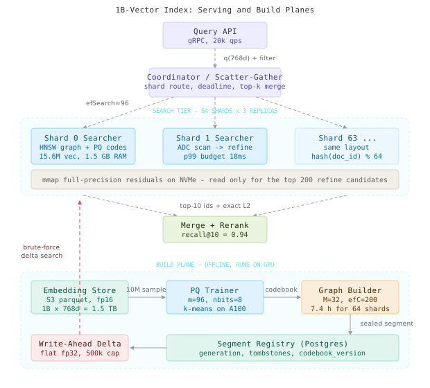
A query arrives at the Query API as a 768-float array plus k and an optional filter predicate. The API normalizes the vector, resolves the filter into a selectivity estimate, and hands off to the Coordinator. The coordinator fans the query out to all 64 shards, asking each for k + 20 results rather than k, because the global top-10 is not evenly distributed across shards and asking for exactly 10 from each loses recall at the merge boundary. Each shard runs its own two-stage search and returns candidate IDs with distances. The coordinator heap-merges 1,920 candidates down to 10 and returns.

Inside a shard, the search is two stages. Stage one traverses the HNSW graph, computing every distance from the 96-byte PQ codes using an asymmetric distance table built once per query. This never loads a full vector from memory, which is the entire point: at efSearch=96 a traversal computes roughly 2,900 distances, and doing that against fp16 vectors would mean touching 4.4 MB of scattered memory instead of 278 KB. Stage two takes the top 200 approximate candidates, fetches their full fp16 vectors from an mmaped file on NVMe, and recomputes exact distances. Reading 300 KB of random NVMe is about 3.1ms, which is affordable once per query but would be ruinous if you did it during traversal.

The build plane reads fp16 embeddings from S3, trains PQ codebooks on a 10M-vector sample, encodes the full corpus, and builds one HNSW graph per shard on GPU. A sealed segment is immutable: three files, an atomic registry row, and a generation number. New writes land in a small flat delta segment that is brute-forced on every query until it is large enough to seal, which is how a vector becomes searchable in under two seconds without touching the sealed graph.

The HNSW Graph Layer

This component’s job is to get from an arbitrary entry point to the neighborhood of the query vector in a few dozen hops instead of a billion comparisons.

HNSW is a skip list where the elements are points in space instead of sorted keys. Every vector lives in layer 0. Each vector is also promoted to layer 1 with probability 1/M, to layer 2 with probability 1/M^2, and so on, so the layers get exponentially sparser as you go up. Search starts at the single entry point in the top layer, greedily walks to the closest node it can find there, drops to the next layer down at that position, and repeats. The top layers are a coarse map that gets you to the right continent; layer 0 is the street grid.

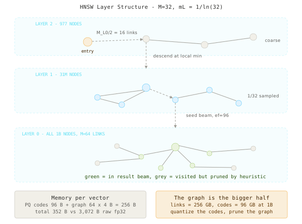
The parameter that people misread is M. It is not a search parameter, it is a build parameter that permanently determines memory. Layer 0 uses 2 * M links per node, higher layers use M. At M=32 with int32 node IDs, layer 0 costs 64 * 4 = 256 bytes per vector in links alone. That is more than the 96 bytes of PQ codes. At a billion vectors, the graph is 256 GB and the codes are 96 GB.

Here is the traversal, written out so the efSearch beam is explicit. This is the core of stage one and it never touches a full vector.

# Layer-0 beam search over PQ codes: the hot loop of every query.
import heapq
import numpy as np

def search_layer_zero(
    query_lut: np.ndarray,        # (m=96, 256) precomputed ADC table, float32
    codes: np.ndarray,            # (n, 96) uint8, RAM resident
    adjacency: np.ndarray,        # (n, 64) int32, -1 padded
    entry_points: list[int],      # seeded from layer 1 descent
    ef: int = 96,
    tombstones: np.ndarray | None = None,   # bool mask, may be None
) -> list[tuple[float, int]]:
    def adc(node: int) -> float:
        # Asymmetric distance: 96 table lookups, 96 adds, no vector load.
        return float(query_lut[np.arange(96), codes[node]].sum())

    visited = set(entry_points)
    # candidates: min-heap by distance, the frontier we still want to expand
    candidates: list[tuple[float, int]] = []
    # results: max-heap by negated distance, the best ef found so far
    results: list[tuple[float, int]] = []

    for ep in entry_points:
        d = adc(ep)
        heapq.heappush(candidates, (d, ep))
        heapq.heappush(results, (-d, ep))

    while candidates:
        d_cand, node = heapq.heappop(candidates)
        worst_result = -results[0][0]
        # The termination condition that makes HNSW sublinear: once the closest
        # unexpanded candidate is farther than our worst keeper, stop.
        if d_cand > worst_result and len(results) >= ef:
            break

        for neighbor in adjacency[node]:
            if neighbor < 0 or neighbor in visited:
                continue
            visited.add(int(neighbor))
            d = adc(int(neighbor))
            worst_result = -results[0][0]
            if len(results) < ef or d < worst_result:
                heapq.heappush(candidates, (d, int(neighbor)))
                heapq.heappush(results, (-d, int(neighbor)))
                if len(results) > ef:
                    heapq.heappop(results)

    out = [(-d, node) for d, node in results]
    if tombstones is not None:
        out = [(d, n) for d, n in out if not tombstones[n]]
    out.sort()
    return out

The subtle part is the break condition. HNSW is sublinear precisely because it stops expanding as soon as the nearest unexplored candidate is worse than the worst result it is already holding. Remove that check and the beam search degenerates into a breadth-first flood of the whole graph. Keep the check but set ef too low and the beam collapses into a greedy walk that gets stuck in a local minimum, which is exactly what produces recall@10 of 0.34 at the library defaults.

What breaks if we simplify? Drop the hierarchy and keep only layer 0, and you have NSW: it still works, but the entry point is random, so the walk needs roughly log(n) more hops to escape a bad starting region. At a billion vectors that measured out at 3.8x more distance computations for the same recall. The hierarchy is not about the graph’s quality, it is about the cost of getting to the right part of it.