Build a Disaggregated Prefill-Decode Inference Architecture


performance scalability caching

AI System Design Deep Dive

Disaggregated Prefill-Decode

Prefill wants raw compute. Decode wants steady memory bandwidth. Never make one GPU do both.

⏱ 14 min read📐 Advanced🧠 LLM Inference

A print shop running a single press for both jobs learns this the hard way: the offset run for a 5,000-copy flyer needs the whole machine flat out for twenty minutes, while the letterpress job next to it needs the same machine free for six hours, one impression every few seconds, never fully loaded but never allowed to stop either. Put both jobs on one press and you get the worst of both schedules. LLM inference has the same two jobs living on one GPU, and it has for years: prefill, which reads the entire prompt and computes attention over all of it in one dense, compute-bound burst, and decode, which then generates one token at a time in a loop that is bound almost entirely by how fast you can read the KV cache back out of memory.

Prefill wants big batches and every tensor core saturated. Decode wants low latency per step and enough free memory to hold hundreds of concurrent KV caches. When both run on the same GPU, a single long prompt arriving mid-stream stalls every other user’s decode step behind it, because the scheduler has to finish the compute-heavy prefill pass before it can resume the memory-bound decode pass. This is the co-located serving tax: at 5 requests/second on one A100, nobody notices. At 5,000 requests/second across a shared pool, prefill interference becomes the dominant source of tail latency, and no amount of batching tuning fixes it, because the problem isn’t the scheduler, it’s that one physical GPU is being asked to be two different machines at once.

The fix is architectural, not algorithmic: put prefill and decode on separate GPU pools, sized and provisioned for their own workload shape, and move the computed KV cache between them over a fast interconnect once prefill finishes. Prefill nodes can now run at high batch sizes tuned purely for compute throughput. Decode nodes can now run continuous batching tuned purely for TPOT (time-per-output-token) stability, free of prefill interference. The catch is that this turns a local memory copy into a network transfer, and that transfer has to complete inside the latency budget you were trying to protect in the first place.

We need to solve for three things simultaneously: routing each incoming request to the right prefill node without creating a hot spot, transferring gigabytes of KV cache blocks across the network fast enough that the decode node never idles waiting for them, and sizing the two pools independently so neither one is starved while the other sits idle.

Key Insight

Disaggregation doesn’t remove work, it moves a memory copy that used to be free (same GPU, same HBM) onto a network link that has to be fast enough to be invisible. The entire design lives or dies on that transfer path.

Requirements and Constraints

Functional Requirements

  • Accept a completion request, run prefill on a dedicated prefill-tier GPU, and produce the first token and the full KV cache for the prompt
  • Transfer the computed KV cache blocks to an assigned decode-tier GPU without re-computing them
  • Resume generation on the decode tier using the transferred cache, streaming tokens back to the client via SSE
  • Support prompts long enough to require chunked prefill so a single 32k-token prompt does not monopolize a prefill GPU for multiple seconds
  • Support multi-turn conversations where a follow-up turn can reuse KV cache already resident on a decode node (prefix cache hit) without a fresh transfer
  • Rebalance load across both pools independently as request mix shifts between prefill-heavy (long prompts, short answers) and decode-heavy (short prompts, long answers) traffic

Non-Functional Requirements

  • Latency: time-to-first-token (TTFT) p99 under 150ms for prompts up to 2k tokens, including transfer time; time-per-output-token (TPOT) p99 under 30ms once decode starts
  • Throughput: sustain 12,000 aggregate decode tokens/second across the decode pool at 500 concurrent sequences average
  • Transfer: KV cache transfer must complete in under 40ms for a 2k-token prompt on Llama-3 70B (roughly 900 MB of KV blocks) to stay inside the TTFT budget
  • Quality: zero degradation versus co-located serving. Disaggregation is a performance and cost change, not an accuracy change, so output tokens must be bit-identical given the same sampling seed
  • Cost: GPU-hours per million output tokens must drop versus co-located serving, since prefill GPUs no longer sit idle waiting for decode loops to catch up
  • Capacity: decode-tier GPU memory is the binding constraint, since it holds hundreds of concurrent KV caches; prefill-tier GPU memory only needs to hold the batch currently being processed plus the model weights

Constraints

  • Assume Llama-3 70B in FP16 or BF16 as the served model, tensor parallelism degree 4 per replica on both tiers
  • Assume 8xH100 80GB nodes with NVLink inside a node and RDMA over InfiniBand (RoCEv2) between nodes
  • Assume a transfer engine capable of GPU-direct RDMA (no CPU staging copy) is available, either a custom implementation or an existing one such as NIXL or Mooncake’s transfer engine
  • Out of scope: multi-modal inputs, speculative decoding, and fine-tuning workloads. This design is serving-only
  • Out of scope: cross-region disaggregation. Prefill and decode pools live in the same data center on the same RDMA fabric

High-Level Architecture

The system has five major components. The Global Scheduler accepts requests and assigns each one to a prefill node and, once prefill finishes, to a decode node. The Prefill Pool is a set of GPU replicas tuned for high-batch compute throughput, running chunked prefill so long prompts don’t block the queue. The Transfer Engine moves KV cache blocks from a prefill node’s HBM directly into a decode node’s HBM over RDMA, without a CPU-side copy. The Decode Pool is a separate set of GPU replicas running continuous batching, receiving already-computed KV caches and generating tokens against them. The KV Block Directory is a metadata service, backed by Redis, that tracks which physical GPU and block offsets currently own each sequence’s KV cache, so the scheduler and transfer engine always know where data lives.
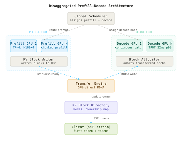
Disaggregated prefill-decode architecture showing the global scheduler routing requests between a prefill pool and a decode pool, connected by a KV cache transfer engine over RDMA, with a block directory tracking cache ownership

A request arrives at the Global Scheduler, which checks the KV Block Directory for a prefix cache hit (a returning conversation whose earlier turns are still resident on some decode node), then assigns the request to the least-loaded prefill replica. The prefill replica runs the forward pass over the prompt, writes KV blocks into its own paged memory pool, and signals completion. The Transfer Engine then pulls those blocks directly across RDMA into a decode replica chosen by the scheduler for having headroom in its KV cache budget, updates the KV Block Directory with the new owner, and hands control to the decode replica’s continuous batching loop, which starts streaming tokens back to the client over SSE.

Key Insight

The single most important decision in this architecture is making the transfer asynchronous and pipelined with the tail of prefill, not a hard barrier after it. The decode node reserves KV cache space and starts pulling the earliest completed blocks while the prefill node is still writing the last few, so the transfer’s critical path is milliseconds, not the full block size divided by bandwidth.

The Global Scheduler

The scheduler’s job is to decide, for every request, which prefill node computes it and which decode node continues it, without letting either pool develop a hot spot.

A naive round-robin assignment looks fine until traffic mixes long prompts with short ones. A prefill node that just got handed three 16k-token prompts in a row is now the slowest node in the pool for the next several seconds, and round-robin keeps sending it more work anyway because it doesn’t know that.

Watch Out

Round-robin or random assignment across the prefill pool looks correct in low-traffic testing and then produces a persistent tail-latency cluster in production the moment prompt length variance increases, because it has no concept of “how much work is already queued here.”

The fix is queue-depth-aware assignment: each prefill node reports its current queued token count (not request count, token count) every scheduling tick, and the scheduler picks the node with the least queued work, weighted by expected prefill compute cost, which scales roughly with prompt length squared for attention but is dominated by the linear KV write cost in practice for chunked prefill implementations. On the decode side, assignment is driven by available KV cache budget, not request count, since a decode node holding fewer but longer-context sequences can be just as full as one holding many short ones.

# Scheduler assignment logic: picks prefill and decode targets by load, not round-robin
import asyncio
from dataclasses import dataclass

@dataclass
class NodeLoad:
    node_id: str
    queued_tokens: int
    kv_cache_used_bytes: int
    kv_cache_capacity_bytes: int

class GlobalScheduler:
    def __init__(self, prefill_nodes: list[NodeLoad], decode_nodes: list[NodeLoad]):
        self.prefill_nodes = prefill_nodes
        self.decode_nodes = decode_nodes
        self._lock = asyncio.Lock()

    async def pick_prefill_node(self, prompt_tokens: int) -> str:
        async with self._lock:
            best = min(self.prefill_nodes, key=lambda n: n.queued_tokens)
            best.queued_tokens += prompt_tokens
            return best.node_id

    async def pick_decode_node(self, est_kv_bytes: int) -> str | None:
        async with self._lock:
            candidates = [
                n for n in self.decode_nodes
                if n.kv_cache_capacity_bytes - n.kv_cache_used_bytes >= est_kv_bytes
            ]
            if not candidates:
                return None
            best = min(candidates, key=lambda n: n.kv_cache_used_bytes / n.kv_cache_capacity_bytes)
            best.kv_cache_used_bytes += est_kv_bytes
            return best.node_id

    def release_prefill_load(self, node_id: str, prompt_tokens: int) -> None:
        for n in self.prefill_nodes:
            if n.node_id == node_id:
                n.queued_tokens = max(0, n.queued_tokens - prompt_tokens)

What would break if you simplified this to plain round-robin: tail latency at p99 would track the longest prompt in the last N requests instead of tracking system-wide load, because one unlucky node absorbs a burst of long prompts and stays hot long after the burst passes. The failure mode is silent, it never errors, it just slowly inflates p99 TTFT until someone notices the SLA dashboard.

Real World

NVIDIA Dynamo (formerly Triton’s disaggregated serving mode) and the DistServe research system both use load-aware placement across prefill and decode pools rather than static assignment, precisely because prompt length variance in production traffic makes static routing degrade within minutes of real load.

The Prefill Pool

Each prefill replica’s job is to turn a prompt into a KV cache as fast as possible, then get out of the way.

The non-obvious part: a smart engineer’s first instinct is to give the prefill pool the biggest possible batch size, since prefill is compute-bound and batching amortizes fixed costs. That’s right for throughput but wrong for latency, because a max-size prefill batch containing one 20k-token prompt can take 2 to 3 seconds to complete on an H100, during which no other prompt in that batch gets a head start. Chunked prefill fixes this by splitting long prompts into fixed-size chunks (commonly 2k to 4k tokens) and interleaving those chunks with other prompts’ prefill work, so no single long prompt monopolizes a GPU for multiple seconds.

Prefill pool internals showing chunked prefill splitting a long prompt into fixed-size chunks interleaved with shorter prompts in the same batch, plus the KV block writer feeding the transfer queue
# Chunked prefill batch builder: caps per-iteration prefill tokens so no single prompt stalls the queue
from dataclasses import dataclass, field

MAX_PREFILL_TOKENS_PER_ITER = 4096

@dataclass
class PrefillRequest:
    request_id: str
    tokens: list[int]
    cursor: int = 0

    @property
    def remaining(self) -> int:
        return len(self.tokens) - self.cursor

    def next_chunk(self, budget: int) -> list[int]:
        take = min(budget, self.remaining)
        chunk = self.tokens[self.cursor:self.cursor + take]
        self.cursor += take
        return chunk

def build_prefill_batch(queue: list[PrefillRequest]) -> dict[str, list[int]]:
    budget = MAX_PREFILL_TOKENS_PER_ITER
    batch: dict[str, list[int]] = {}
    for req in sorted(queue, key=lambda r: r.remaining):
        if budget <= 0:
            break
        chunk = req.next_chunk(min(budget, req.remaining))
        if chunk:
            batch[req.request_id] = chunk
            budget -= len(chunk)
    return batch

Scheduling shortest-remaining-work first inside the chunk budget is a small change with an outsized effect: it means short prompts finish and start streaming almost immediately, while long prompts get steady progress across several iterations instead of blocking everything until they’re fully done. This is the same shortest-job-first intuition that keeps interactive workloads responsive on a shared CPU scheduler, applied to token budgets instead of CPU time slices.

Watch Out

Without chunked prefill, disaggregation still helps decode-side interference, but the prefill pool itself becomes the new tail-latency source: a burst of long documents queued for RAG or summarization can push TTFT for every other request behind them into the seconds range.

The Transfer Engine

The transfer engine’s job is to move a completed KV cache from prefill-tier HBM to decode-tier HBM fast enough that it never becomes the dominant term in TTFT.

The obvious approach, copy KV blocks to host memory on the prefill node then send over TCP then copy back into GPU memory on the decode node, has three memory copies and a kernel-mediated network stack in the critical path. At 900MB per transfer (Llama-3 70B, 2k-token prompt) even at a generous 10GB/s effective TCP throughput, that’s 90ms just for the wire transfer, before either copy. That alone blows most of the 150ms TTFT budget.

Cost Math

GPU-direct RDMA over a 200Gb/s (25GB/s) InfiniBand link moves that same 900MB in about 36ms with zero CPU copies. The naive TCP-plus-staging path costs roughly 3x the latency and pins a CPU core on both ends for the memcopy, which is GPU-hours you paid for sitting idle waiting on a network stack.

The fix is a transfer engine that registers GPU memory regions for RDMA directly (no host staging), and pipelines the transfer with the tail of prefill computation rather than waiting for the whole prefill pass to complete before starting any transfer. As soon as the first few KV blocks are written, they’re eligible to start moving.

# Transfer engine: pipelines block transfer with prefill completion, GPU-direct RDMA
import asyncio
from dataclasses import dataclass

@dataclass
class KVBlock:
    block_id: int
    gpu_ptr: int
    size_bytes: int
    ready: bool = False

class TransferEngine:
    def __init__(self, rdma_endpoint):
        self.rdma = rdma_endpoint

    async def stream_transfer(self, blocks: list[KVBlock], dest_node: str, dest_ptrs: list[int]):
        # transfer each block the instant it's marked ready by the prefill writer
        pending = list(zip(blocks, dest_ptrs))
        in_flight = []
        while pending:
            ready_now = [(b, d) for b, d in pending if b.ready]
            for block, dest_ptr in ready_now:
                in_flight.append(asyncio.create_task(
                    self.rdma.write(
                        src_ptr=block.gpu_ptr,
                        dst_node=dest_node,
                        dst_ptr=dest_ptr,
                        size=block.size_bytes,
                    )
                ))
                pending.remove((block, dest_ptr))
            if in_flight:
                done, in_flight = await asyncio.wait(in_flight, timeout=0.001, return_when=asyncio.FIRST_COMPLETED)
            else:
                await asyncio.sleep(0.0005)
        if in_flight:
            await asyncio.wait(in_flight)
Token flow from prompt ingestion through chunked prefill, pipelined RDMA block transfer, and continuous decode, showing the KV cache moving from prefill GPU memory to decode GPU memory while the first token streams to the client

What breaks if you drop the pipelining and just wait for full prefill completion before starting any transfer: TTFT becomes prefill_time + full_transfer_time strictly in series, instead of mostly overlapped. For a 2k-token prompt that’s the difference between roughly 60ms (overlapped) and 130ms (serial) on the transfer contribution alone, which is most of your latency budget for one design choice.

Real World

Moonshot AI’s Mooncake, used to serve Kimi at scale, and NVIDIA’s NIXL transfer library both implement GPU-direct, pipelined KV transfer for exactly this reason. Mooncake’s public writeup reports the transfer engine sustaining near-line-rate RDMA throughput for KV cache movement, which is what makes their disaggregated prefill-decode split viable in production rather than just a paper result.

The Decode Pool

Each decode replica’s job is to run continuous batching against KV caches it did not compute itself, generating one token per sequence per iteration.

This is where a subtle correctness requirement shows up: the decode replica must reconstruct the exact paged memory layout the prefill replica used, block for block, or attention will read garbage. The KV Block Directory doesn’t just track which node owns which sequence, it tracks the block table (the mapping from logical sequence position to physical block index) so the decode node can allocate matching physical blocks and receive the transfer into the right addresses.

# Decode-side admission: allocates matching block layout before accepting an incoming transfer
from dataclasses import dataclass

BLOCK_SIZE_TOKENS = 16

@dataclass
class BlockTable:
    sequence_id: str
    physical_blocks: list[int]

class DecodeBlockAllocator:
    def __init__(self, total_blocks: int):
        self.free_blocks = list(range(total_blocks))
        self.tables: dict[str, BlockTable] = {}

    def admit(self, sequence_id: str, num_tokens: int) -> BlockTable | None:
        needed = (num_tokens + BLOCK_SIZE_TOKENS - 1) // BLOCK_SIZE_TOKENS
        if len(self.free_blocks) < needed:
            return None  # signal scheduler to pick a different decode node
        allocated = [self.free_blocks.pop() for _ in range(needed)]
        table = BlockTable(sequence_id=sequence_id, physical_blocks=allocated)
        self.tables[sequence_id] = table
        return table

    def release(self, sequence_id: str) -> None:
        table = self.tables.pop(sequence_id, None)
        if table:
            self.free_blocks.extend(table.physical_blocks)

Once caches land, the decode loop is standard continuous batching: every iteration, run one forward pass across all active sequences, emit one token each, evict sequences that hit <eos> or their max length, and admit newly-arrived transferred sequences into the freed slots. The difference from co-located serving is that this loop never has to interleave a compute-bound prefill chunk with decode steps, so its per-iteration latency is far more predictable.

Key Insight

TPOT variance, not average TPOT, is what disaggregation actually fixes. Average tokens/second on a co-located pool can look fine in aggregate while individual users experience a stutter every time a long prompt lands in their batch. Separating the pools removes the stutter, not just the average.

Watch Out

If decode-side admission fails (no free blocks) after prefill already finished and transfer already started, you’ve burned prefill compute and network bandwidth for nothing. Reserve decode capacity before starting the transfer, not after, and have the scheduler re-check availability at assignment time, not at transfer-start time.

Data Model

The system tracks three kinds of state: relational metadata about requests and nodes, the KV block ownership directory, and transfer event records for observability.

-- Core relational schema: requests, node registry, and transfer audit log
CREATE TABLE inference_requests (
    request_id       UUID PRIMARY KEY,
    tenant_id         UUID NOT NULL,
    prompt_tokens     INT NOT NULL,
    prefill_node_id   TEXT NOT NULL,
    decode_node_id    TEXT,
    status            TEXT NOT NULL CHECK (status IN ('prefilling', 'transferring', 'decoding', 'done', 'failed')),
    ttft_ms           INT,
    created_at        TIMESTAMPTZ NOT NULL DEFAULT now(),
    completed_at      TIMESTAMPTZ
);
CREATE INDEX idx_requests_status ON inference_requests (status, created_at);
CREATE INDEX idx_requests_tenant ON inference_requests (tenant_id, created_at DESC);

CREATE TABLE gpu_nodes (
    node_id           TEXT PRIMARY KEY,
    pool              TEXT NOT NULL CHECK (pool IN ('prefill', 'decode')),
    tp_degree         INT NOT NULL,
    kv_capacity_bytes BIGINT NOT NULL,
    kv_used_bytes     BIGINT NOT NULL DEFAULT 0,
    queued_tokens     INT NOT NULL DEFAULT 0,
    last_heartbeat    TIMESTAMPTZ NOT NULL DEFAULT now()
);

CREATE TABLE kv_transfer_events (
    transfer_id       UUID PRIMARY KEY,
    request_id        UUID NOT NULL REFERENCES inference_requests(request_id),
    src_node_id       TEXT NOT NULL,
    dst_node_id       TEXT NOT NULL,
    bytes_transferred BIGINT NOT NULL,
    duration_ms       INT NOT NULL,
    started_at        TIMESTAMPTZ NOT NULL,
    finished_at       TIMESTAMPTZ
);

The KV Block Directory itself is a Redis structure, not the relational store, because it is on the hot path for every scheduling decision and every transfer, and needs sub-millisecond lookups:

HSET blockdir:req:8f3a "src_node" "prefill-04" "dst_node" "decode-11" "block_count" "72" "status" "transferring"
EXPIRE blockdir:req:8f3a 120
SADD nodeload:decode-11:sequences "8f3a"

Partitioning key choice here is the request ID for the directory (each entry is independent and short-lived) and the node ID for the relational gpu_nodes table (one row per physical replica, updated on every heartbeat). There is no vector index in this system since it serves raw completions, not retrieval, so indexing strategy is limited to the two B-tree indexes above plus the Redis hash TTL, which auto-expires stale directory entries if a transfer fails silently.

Lifecycle of a request record moving through prefilling, transferring, decoding, and done states, with the KV block directory entry created at prefill start and released at decode completion

Key Algorithms and Protocols

Chunked Prefill Scheduling

Already covered above in the prefill pool section. The complexity is O(n log n) per scheduling tick for the sort by remaining tokens, which is negligible next to the O(chunk_size^2) attention cost it’s protecting.

Pipelined RDMA Block Streaming

The core property that makes this work at scale is overlap, not raw bandwidth. A transfer engine that waits for prefill to fully complete before starting any block writes gets zero benefit from a faster network, since the critical path is still prefill_time + transfer_time in series. A pipelined engine gets max(prefill_time, transfer_time) plus a small tail, because most of the transfer overlaps with the tail of compute.

Key Insight

The property that makes pipelined transfer correct under concurrency is per-block readiness signaling, not a single “prefill done” flag. Each KV block must independently report ready so the transfer engine can start moving early blocks while later ones are still being written, without any risk of transferring a partially-written block.

Continuous Batching on the Decode Side

Standard admit-evict-per-iteration scheduling, identical in principle to a co-located continuous batching server, except the admission source is transferred caches instead of freshly prefilled ones. Time complexity per iteration is O(active_sequences), space is bounded by kv_capacity_bytes per node, which is the actual ceiling on concurrency.

Edge case worth naming explicitly: a sequence whose transfer partially completes before a network fault (RDMA link flap) must be detected and either retried from the prefill node’s still-resident cache, or the whole request re-prefilled from scratch if the prefill node has already evicted it. The directory’s status = 'transferring' with no update past a timeout is the detection signal.

# Transfer stall detector: reissues or fails a request whose transfer has stalled past SLA
import time

TRANSFER_STALL_MS = 200

def check_stalled_transfers(directory_entries: list[dict]) -> list[str]:
    now_ms = time.time() * 1000
    stalled = []
    for entry in directory_entries:
        if entry["status"] == "transferring":
            elapsed = now_ms - entry["started_at_ms"]
            if elapsed > TRANSFER_STALL_MS:
                stalled.append(entry["request_id"])
    return stalled

Scaling and Performance

Prefill and decode pools now scale independently, which is the entire point, but each has its own ceiling. A single prefill replica’s throughput ceiling is bounded by tensor core utilization at its chosen batch size, and adding more replicas scales throughput linearly as long as the scheduler keeps load balanced. A single decode replica’s ceiling is bounded by KV cache capacity in HBM, since that determines how many concurrent sequences it can hold, and that ceiling does not move by adding compute, only by adding memory or shrinking the cache per sequence.

Scaling diagram showing independent horizontal scaling of the prefill pool and decode pool, with the KV cache capacity ceiling on decode nodes and compute ceiling on prefill nodes as the two distinct bottlenecks
Given:
  - Llama-3 70B, TP degree 4, BF16 weights = 140 GB across 4 GPUs (35 GB/GPU)
  - 8xH100 80GB node, TP=4 means 2 replicas per node
  - KV cache per token = 2 * 80 layers * 8 kv heads * 128 head_dim * 2 bytes = 327,680 bytes = ~0.33 MB/token
  - Target: 500 concurrent decode sequences, avg 2,200 tokens context (prompt + generated so far)

Per-GPU usable memory for KV cache: 80 GB - 35 GB weights - ~5 GB activations = ~40 GB
KV cache per sequence: 2,200 tok * 0.33 MB = ~726 MB = 0.71 GB
Concurrent seqs per decode replica: 40 GB / 0.71 GB = ~56
Decode replicas needed for 500 concurrent seqs: 500 / 56 = ~9 replicas = ~5 nodes (2 replicas/node)

Prefill throughput needed: 500 req/s arrival * 900 avg prompt tokens = 450,000 prefill tokens/s
Single prefill replica (H100, TP=4, chunked at 4096 tok/iter) sustains ~28,000 prefill tokens/s
Prefill replicas needed: 450,000 / 28,000 = ~17 replicas = ~9 nodes

The decode pool ends up smaller in node count here but each node is fully memory-bound, while the prefill pool needs more replicas because arrival-rate-driven prefill demand outpaces what a handful of compute-bound replicas can chew through. This ratio flips for workloads with long prompts and short answers (RAG-style traffic), which is exactly why sizing the two pools independently, instead of a fixed ratio, matters.

The transfer path itself is the read/write hot spot to watch: every completed prefill writes once and every decode admission reads once, so transfer bandwidth scales linearly with request rate, not with pool size. At 500 req/s and ~700MB average transfer size, aggregate transfer bandwidth demand is roughly 350 GB/s, which is why the RDMA fabric, not GPU compute, is the resource you monitor most closely as traffic grows.

Real World

The DistServe paper reports that disaggregation lets each pool hit its own goodput ceiling independently, and in their evaluated configurations this raised achievable per-GPU goodput by roughly 2x to 4x over the best co-located configuration at the same latency SLA, because neither pool had to compromise its batching strategy to accommodate the other’s workload shape.

Cost and Token Economics

The dollar case for disaggregation rests on GPU utilization shape, not raw hardware savings. Co-located GPUs waste cycles two ways: prefill bursts stall decode progress (wasted decode-node time), and decode’s steady but modest compute demand under-utilizes tensor cores that a dedicated prefill node would keep saturated.

ConfigurationGPU-hours / 1M output tokensp99 TTFTp99 TPOTNotes
Co-located, static batching0.581,900ms48msbaseline, no disaggregation
Co-located, continuous batching0.41620ms32msgood scheduler, same GPU pool
Disaggregated, unpipelined transfer0.36410ms24mstransfer engine adds latency but pools no longer starve each other
Disaggregated, pipelined RDMA transfer0.27145ms22mstransfer overlaps prefill tail, near-zero added latency

The measured optimization here is the pipelined transfer engine specifically: moving from unpipelined to pipelined RDMA transfer cut p99 TTFT by roughly 65% with no change to GPU count, purely by removing the serialization between prefill completion and transfer start. That’s the single highest-leverage change in the whole design, because it’s the only lever that improves both cost and latency at the same time rather than trading one for the other.

Cost Math

Going from co-located static batching to disaggregated pipelined transfer cuts GPU-hours per million output tokens by roughly 53% (0.58 down to 0.27) while also cutting p99 TTFT by 92%. At $3.20/GPU-hour for H100 on-demand pricing, that’s a swing from roughly $1.86 to $0.86 per million output tokens, which compounds fast at real traffic volumes.

Quality, Evaluation, and Guardrails

Disaggregation is a performance change, not a model change, so the quality bar is correctness equivalence: given the same prompt, sampling parameters, and seed, a disaggregated request must produce token-identical output to a co-located request. Any divergence signals a bug in block layout reconstruction, not a model quality issue, and needs to gate deploys the same way a broken build would.

The offline eval here is a golden set of prompts run through both a co-located reference server and the disaggregated pipeline, diffed token-by-token. Online, the signal is a low-rate shadow comparison: a small percentage of live traffic gets mirrored to both paths and compared asynchronously, without blocking the user-facing response.

# Guardrail: verifies token-level equivalence between disaggregated and reference decode paths
def verify_token_equivalence(reference_tokens: list[int], disaggregated_tokens: list[int]) -> dict:
    mismatches = [
        i for i, (r, d) in enumerate(zip(reference_tokens, disaggregated_tokens)) if r != d
    ]
    length_mismatch = len(reference_tokens) != len(disaggregated_tokens)
    return {
        "match": not mismatches and not length_mismatch,
        "first_mismatch_index": mismatches[0] if mismatches else None,
        "length_mismatch": length_mismatch,
    }

The threshold that triggers rollback is any non-zero mismatch rate above sampling-induced noise (there is none here since seeds are fixed for the eval set), so in practice the gate is: zero tolerance on the golden set, and an automatic page if shadow-traffic mismatch rate exceeds 0.1% over a rolling 15-minute window, since anything above that almost certainly indicates a block table bug, not a fluke.

Watch Out

The silent regression to watch for is subtle KV block misalignment: attention over slightly wrong block offsets doesn’t crash, it produces plausible-looking but wrong tokens, especially in long-context conversations where a small transfer bug only manifests after several turns. This fails softly and will not show up in short smoke tests.

Failure Modes and Recovery

FailureDetectionImpactRecovery
RDMA link flap mid-transfertransfer stall timeout (no directory update past 200ms)affected request stalls, others unaffectedretry from prefill node’s still-resident cache; if evicted, re-prefill from scratch
Decode node OOM on admissionallocator returns no free blocksrequest cannot be admitted to that nodescheduler picks a different decode node before starting transfer, never after
Prefill node crash mid-chunkheartbeat miss on gpu_nodes tablein-flight prompts on that node lostrequests re-queued to next-best prefill node, client sees added latency, not an error
KV Block Directory entry expires before decode completesTTL fires on Redis key while status is not donescheduler loses track of ownershipdirectory writes refresh TTL on every heartbeat from the owning node; expiry without refresh is treated as node-dead
Prefix cache hit references evicted blocksdecode node reports missing block IDs on lookupconversation continuation fails prefix reusefall back to full re-prefill of prior turns, transparent to the client, slower but correct
Transfer engine backlog under traffic spikeRDMA queue depth exceeds watermarkTTFT degrades across the boardadmission control throttles new prefill starts until backlog drains, protecting in-flight requests
Watch Out

The most common operational mistake is treating the transfer engine as infrastructure plumbing that doesn’t need its own alerting. It needs the same first-class monitoring as the model servers: queue depth, per-transfer latency percentiles, and retry rate, because it sits directly in the TTFT critical path and failures there look identical to “the model is slow” from a dashboard three layers up.

Comparison of Approaches

ApproachLatency (p99 TTFT)Cost (GPU-hr/1M tok)ComplexityFailure modeBest fit
Co-located, static batching~1,900ms0.58LowPrefill blocks decode for entire batch durationLow-traffic prototypes, no SLA pressure
Co-located, continuous batching~620ms0.41MediumLong prompts still cause TPOT stutter for co-scheduled sequencesModerate traffic, single-tenant, simpler ops preferred
Disaggregated, unpipelined transfer~410ms0.36HighTransfer serializes after prefill, eating into TTFT budgetTeams validating disaggregation before investing in a pipelined engine
Disaggregated, pipelined RDMA transfer~145ms0.27Very HighTransfer engine itself becomes a new failure domain requiring dedicated monitoringHigh-traffic production serving with strict TTFT SLAs

For most teams past the prototype stage and serving real traffic with a latency SLA, disaggregated with pipelined RDMA transfer is the right call despite the added operational surface, because the cost and latency gains compound at scale and the added complexity (transfer engine, block directory, independent pool autoscaling) is a one-time investment that pays for itself in reduced GPU spend within weeks at meaningful traffic. Teams still validating product-market fit or running under 100 req/s are usually better served by co-located continuous batching, since the operational overhead of a second GPU pool and a transfer fabric isn’t justified yet.

Scaling and Performance Notes on Autoscaling

Independent pool autoscaling means two separate signals drive scale-out: prefill pool scales on queued token backlog, decode pool scales on aggregate KV cache utilization percentage. A naive shared autoscaler that scales both pools together on request rate alone will consistently over-provision one pool and under-provision the other, since prefill and decode demand shift independently as the prompt-length-to-completion-length ratio changes across the traffic mix throughout the day.

Key Insight

Track the ratio of prefill-bound to decode-bound demand as its own metric, not just aggregate QPS. A sudden shift toward long-document summarization traffic needs more prefill replicas with no change to decode capacity, and a naive QPS-based autoscaler cannot see that distinction.

Key Takeaways

  • Disaggregation separates prefill’s compute-bound workload from decode’s memory-bound workload onto physically distinct GPU pools, eliminating the interference that caps co-located serving’s tail latency.
  • Chunked prefill caps how many tokens of a single prompt enter one scheduling iteration, preventing a long document from monopolizing an entire prefill replica.
  • Pipelined RDMA transfer overlaps KV cache movement with the tail of prefill compute, turning what would be a serial latency addition into a near-invisible parallel step.
  • The KV Block Directory is the source of truth for cache ownership and must be on the hot path with sub-millisecond lookups, since every scheduling and transfer decision depends on it.
  • Independent pool autoscaling driven by queued tokens (prefill) and KV cache utilization (decode) outperforms a shared QPS-based autoscaler, since the two pools’ demand shifts independently with traffic mix.
  • GPU-direct RDMA removes the CPU staging copy that would otherwise dominate transfer latency, making the difference between a 36ms and a 130ms transfer for a 2k-token prompt.
  • Correctness equivalence with co-located serving, not new capability, is the quality bar. Any token-level divergence signals a block layout bug, not a model quality tradeoff.
  • Transfer engine health needs first-class monitoring, because it sits directly in the TTFT critical path and its failures masquerade as generic model slowness.

The counter-intuitive lesson: disaggregation looks like it should add latency, since you’ve inserted a network hop into a path that used to be a free memory access on the same GPU. It ends up reducing latency instead, because removing prefill interference from the decode loop is worth more than the transfer costs, as long as that transfer is pipelined rather than serial. The architecture wins by trading a small, well-controlled cost (RDMA transfer) for eliminating a large, unpredictable one (batch interference).

Frequently Asked Questions

Q: Why not just add more GPUs to a co-located pool instead of disaggregating? A: More co-located GPUs increase aggregate throughput but do not fix interference, since every individual replica still runs both prefill and decode and still stalls on long prompts. You’d be paying for hardware to work around a scheduling problem instead of fixing the scheduling problem, and the GPU-hours-per-token cost stays worse than a disaggregated pool at the same total GPU count.

Q: Why RDMA instead of a faster serialization format over regular TCP? A: The bottleneck isn’t serialization, it’s the number of memory copies and the kernel network stack overhead. Even a perfectly efficient TCP payload still requires GPU-to-host and host-to-GPU copies on both ends unless you use GPU-direct RDMA, which writes directly between GPU memory regions across the fabric.

Q: What does this cost to operate versus just using a hosted inference API? A: At high enough sustained volume (roughly above 200-300M tokens/month for a 70B-class model in this analysis), self-hosted disaggregated serving at ~$0.86/1M output tokens undercuts most hosted API pricing for equivalent model quality. Below that volume, the fixed cost of running two GPU pools plus a transfer fabric usually loses to a hosted API’s pay-per-token simplicity.

Q: How do you know the disaggregated path isn’t silently producing worse outputs? A: Token-level equivalence checks against a co-located reference, both offline on a golden set and online via low-rate shadow traffic comparison. Because this is a performance refactor, not a model change, any output divergence is treated as a P1 bug, not a quality regression to tune around.

Q: Why disaggregate prefill and decode instead of disaggregating by tenant or by model version? A: Those are orthogonal and often layered on top of this design, not alternatives to it. Prefill-decode disaggregation solves a workload-shape problem that exists even for a single tenant and a single model version; tenant or model-version isolation solves a blast-radius and rollout problem. Most production systems eventually need both.

Q: What happens to prefix caching (reusing KV cache across conversation turns) in this design? A: It still works, but it changes where the cache lives. A returning conversation’s prior-turn cache is resident on whichever decode node handled the last turn, so the scheduler should prefer routing follow-up turns back to that same decode node to get a local cache hit instead of triggering a fresh cross-pool transfer.

Interview Questions

Q: Walk through what happens, end to end, when a 6,000-token prompt arrives, including every network hop. Expected depth: candidate should trace scheduler assignment, chunked prefill iterations (at 4k tokens/chunk that’s 2 chunks), per-block readiness signaling, pipelined RDMA transfer overlapping the second chunk, decode-side block allocation, and first-token emission, naming where each latency component comes from.

Q: How would you size the decode pool’s KV cache capacity for a target concurrency, and what happens when you get it wrong in each direction? Expected depth: should derive KV bytes per token from model architecture (layers, kv heads, head dim), compute per-sequence cost at expected context length, and explain both failure directions: under-provisioned means admission failures and forced re-routing, over-provisioned means wasted HBM that could hold more concurrent sequences.

Q: The transfer engine’s RDMA link degrades to half bandwidth under a hardware fault. What’s your detection and mitigation strategy? Expected depth: should discuss per-transfer latency percentile monitoring as the detection signal (not just link-level metrics, since those may not directly attribute to affected requests), and mitigation options: admission throttling on the affected fabric segment, failover to a backup RDMA path if available, or temporarily routing new requests to unaffected node pairs.

Q: Why does chunked prefill matter more in a disaggregated architecture than a co-located one? Expected depth: should recognize that in co-located serving, a long prefill at least stalls decode progress for sequences on the same GPU, which is bad but bounded to that replica; in disaggregated serving without chunking, a long prefill blocks the entire prefill pool’s queue since prefill nodes no longer interleave with decode work at all, making the queueing effect pool-wide rather than replica-local.

Q: How would you extend this design to support speculative decoding on the decode tier without touching the prefill tier? Expected depth: should recognize speculative decoding only changes the decode loop’s token-generation step (draft model proposes, target model verifies), so it’s isolated to decode-tier replicas; the interesting design question is whether the draft model needs its own small KV cache budget carved out of the same per-replica HBM, and how that interacts with the concurrency ceiling calculated for the decode pool.

Premium Content

Unlock the full article along with everything else in the archive — all in one place.

In-depth analysis Expert insights Full archive access
Unlock Full Article